Exponential distribution
In probability theory, the exponential distribution describes the time between events in a Poisson point process. It is a continuous probability distribution that serves as a special case of the Gamma distribution. Additionally, it can be considered the continuous counterpart of the geometric distribution.
Table of Contents
- Introduction to Exponential Distribution
- Properties of Exponential Distribution
- Applications of Exponential Distribution
- Importance of Exponential Distribution
- Practical Implementation of Exponential Distribution
- Conclusion
Introduction to Exponential Distribution
In probability theory and statistics, the exponential distribution is a continuous probability distribution commonly used to model the time until a specific event occurs. This distribution is characterized by events occurring independently and at a constant average rate over time. A notable property of the exponential distribution is its memoryless nature, meaning that the probability of an event occurring in the future is independent of how much time has already elapsed.
The values of an exponential random variable tend to be either small or, less frequently, significantly larger. For instance, the amount of money a customer spends during a single visit to a supermarket often follows an exponential distribution.
Exponential Distribution Formula
A continuous random variable X follows an exponential distribution if its probability density function (PDF) is given by:
f(x;λ)= λe−λx x≥0,λ>0
f(x;λ)=0 x>0
Cumulative Distribution Function (CDF)
The cumulative distribution function (CDF) of the exponential distribution is expressed as:
F(x;λ)= 1−e−λx x≥0
F(x;λ)=0 x<0
Properties of Exponential Distribution:
Mean:
![]()
Variance:
![]()
This measures the spread or variability in the time between events.
Memoryless Property
One of the key properties of the exponential distribution is the memoryless property, which is defined as:
P(X>s+t∣X>s)=P(X>t)
for all s,t≥0. This implies that the probability of an event occurring after a certain time interval does not depend on how much time has already passed.
This property implies that the probability of waiting for an additional duration sss is independent of the time that has already passed ttt. In other words, the exponential distribution does not retain memory of previous elapsed time, which is why it is often referred to as "memoryless."
Sum of Two Independent Exponential Random Variables
If X1 and X2are independent exponential random variables with rate parameters λ1 and λ2, then their sum, Z=X1+X2, follows a Gamma distribution. The shape parameter of this Gamma distribution is k=2, and the rate parameter remains λ.
The probability density function (PDF) of Z is given by:
fZ(z)= λ2ze−λz z≥0
fZ(z)=0 z<0
When two independent exponential random variables share the same rate parameter λ, their sum follows a Gamma distribution.
Z~ Gamma(2, λ)
- Mean of the sum: E(Z)=2/λ
- Variance of the sum: Var(Z)=2/λ 2
If the rate parameters are not identical, the sum of the two independent exponential random variables will not follow an exponential distribution. However, it will still adhere to the general form of a Gamma distribution, with its probability density function (PDF) given by:

Cumulative Distribution Function (CDF):
The CDF of an exponential random variable is given by:
![]()
![]()
![]()
![]()
Exponential Distribution Graph
The exponential distribution graph represents the probability density function (PDF), illustrating the distribution of time or distance between occurrences of events. This graph is characterized by two key parameters: lambda (λ) and x.
- λ (Lambda): Represents the rate of events per unit time.
- x: Represents the time between occurrences.
The graph below demonstrates the exponential distribution for different values of λ, such as λ = 1 and λ = 2, showing how the distribution changes based on the event rate.

Applications of the Exponential Distribution
The exponential distribution is extensively used across various domains due to its effectiveness in modeling the time between independent events that occur at a constant rate. Below are some common real-world applications:
1. Reliability Engineering and Failure Prediction
- Use Case: The exponential distribution helps in estimating the time until a mechanical system or an electronic component fails.
- Example: When a device has a constant failure rate, meaning it does not deteriorate over time, the duration between failures follows an exponential distribution.
- Practical Benefit: Engineers can analyze product reliability and predict the Mean Time to Failure (MTTF) for preventive maintenance planning.
2. Queueing Systems and Service Operations
- Use Case: In queueing systems, such as customer service centers, telecommunications, and computing networks, the exponential distribution models the time between arrivals or service durations.
- Example: In a call center, the arrival of customers follows a Poisson process, leading to inter-arrival times that follow an exponential distribution.
- Practical Benefit: Businesses use this to optimize staffing, reduce customer waiting times, and improve service efficiency.
3. Survival Analysis in Medicine
- Use Case: The exponential distribution is applied in medical research to estimate the time until specific events occur, such as disease recurrence or survival duration after treatment.
- Example: The time before a cancer patient experiences a relapse after treatment may follow an exponential distribution.
- Practical Benefit: Helps doctors and healthcare professionals estimate survival probabilities and evaluate treatment effectiveness.
4. Telecommunications and Data Networks
- Use Case: The distribution models the time between data packet arrivals and processing times in communication networks.
- Example: The time between consecutive data packets arriving at a network router can be modeled using an exponential distribution.
- Practical Benefit: Network administrators can efficiently manage bandwidth and optimize data flow for seamless communication.
5. Economics and Business Forecasting
- Use Case: The exponential distribution helps analyze the time between events such as customer purchases, service calls, and stock market transactions.
- Example: In e-commerce, the time gap between successive orders placed by a customer often follows an exponential distribution.
- Practical Benefit: Businesses use this model to predict customer behavior, improve service delivery, and optimize inventory management.
6. Natural Events and Environmental Studies
- Use Case: The distribution models the time interval between unpredictable natural occurrences, such as earthquakes or lightning strikes.
- Example: The time between earthquakes in a specific region can be modeled using an exponential distribution.
- Practical Benefit: Scientists and policymakers can use this model for risk assessment, disaster preparedness, and setting insurance policies.
Importance of the Exponential Distribution
The exponential distribution is fundamental in probability theory and real-world applications due to the following key reasons:
1. Modeling Time Between Events in Poisson Processes
- Significance: It accurately represents the time between random events that occur at a constant average rate.
- Example: In queueing systems, customer arrivals and service requests follow an exponential pattern, helping businesses estimate wait times and optimize resources.
2. Memoryless Property
- Significance: The exponential distribution has a unique "memoryless" characteristic, meaning the probability of an event occurring in the future is independent of how much time has already passed.
- Example: In reliability analysis, this property allows engineers to assume a constant failure rate, simplifying maintenance planning for machines and electronics.
3. Simplicity and Ease of Application
- Significance: The exponential distribution is mathematically simple and easy to apply, relying on just one parameter (λ) for modeling.
- Example: In survival analysis, it provides a quick way to estimate the probability of survival over a given period.
4. Foundation for Advanced Probability Models
- Significance: The exponential distribution serves as a building block for more complex distributions like the gamma distribution (which models the sum of exponential variables) and the Weibull distribution (which extends to variable failure rates).
- Example: When analyzing the total waiting time for multiple independent exponential events, the gamma distribution is used, making this model highly adaptable.
5. Versatility Across Multiple Fields
- Significance: The exponential distribution is applicable in diverse fields such as physics, engineering, economics, medicine, and environmental science.
- Example: In physics, it models radioactive decay, while in finance, it helps in analyzing time gaps between financial transactions.
Implementation of exponential distribution in python
import numpy as np
import matplotlib.pyplot as plt
from scipy.stats import expon
# Set the rate parameter (lambda) for the exponential distribution
lambda_rate = 0.5 # The average time between events is 1/lambda (mean = 2)
# Generate random samples from the exponential distribution
n_samples = 1000
data = expon.rvs(scale=1/lambda_rate, size=n_samples) # scale = 1/lambda
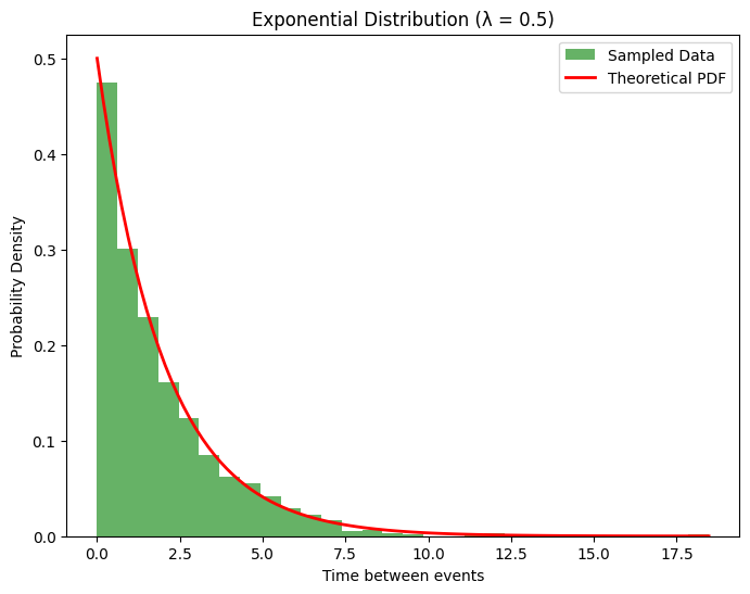
# Plotting the Exponential Distribution
plt.figure(figsize=(8, 6))
plt.hist(data, bins=30, density=True, alpha=0.6, color='g', label='Sampled Data')
# Plotting the theoretical PDF (Probability Density Function)
x = np.linspace(0, np.max(data), 100)
pdf = lambda_rate * np.exp(-lambda_rate * x) # Theoretical PDF
plt.plot(x, pdf, 'r-', lw=2, label='Theoretical PDF')
plt.title(f'Exponential Distribution (λ = {lambda_rate})')
plt.xlabel('Time between events')
plt.ylabel('Probability Density')
plt.legend()
plt.show()
# Mean and Variance calculation
mean = np.mean(data)
variance = np.var(data)
print(f"Mean of the sampled data: {mean:.2f}")
print(f"Variance of the sampled data: {variance:.2f}")
# Memoryless Property demonstration
t = 2 # Given 2 time units have passed, what is the probability event happens after another 2 units
prob = expon.sf(t + t, scale=1/lambda_rate) / expon.sf(t, scale=1/lambda_rate) # P(X > t+s | X > t)
print(f"Probability of event happening after additional 2 units given 2 units have passed: {prob:.2f}")
# Theoretical Mean and Variance
theoretical_mean = 1 / lambda_rate
theoretical_variance = 1 / (lambda_rate ** 2)
print(f"Theoretical Mean: {theoretical_mean:.2f}")
print(f"Theoretical Variance: {theoretical_variance:.2f}")
Mean of the sampled data: 1.93
Variance of the sampled data: 3.87
Probability of event happening after additional 2 units given 2 units have passed: 0.37
Theoretical Mean: 2.00
Theoretical Variance: 4.00
Conclusion:
The exponential distribution plays a vital role in modeling the time intervals between independent events, making it highly applicable in fields such as reliability engineering, queueing theory, and medical survival studies. Its distinct memoryless property and straightforward mathematical structure make it an effective tool for analyzing processes where events happen at a consistent rate. The importance of this distribution stems from its versatility, ease of interpretation, and adaptability, serving as a foundation for more advanced probability models.
Featured Blogs
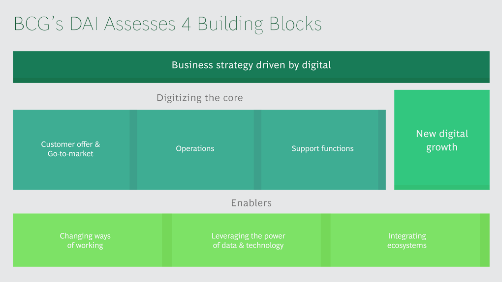
BCG Digital Acceleration Index

Bain’s Elements of Value Framework
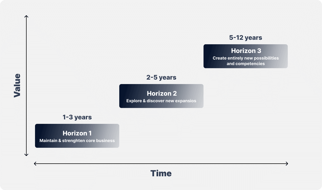
McKinsey Growth Pyramid
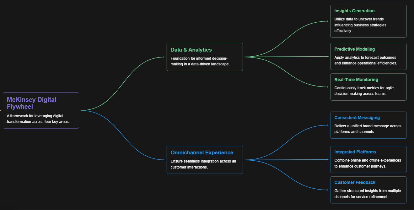
McKinsey Digital Flywheel

McKinsey 9-Box Talent Matrix

McKinsey 7S Framework

The Psychology of Persuasion in Marketing

The Influence of Colors on Branding and Marketing Psychology

What is Marketing?
Recent Blogs

Part 8: From Blocks to Brilliance – How Transformers Became Large Language Models (LLMs) of the series - From Sequences to Sentience: Building Blocks of the Transformer Revolution
Part 7: The Power of Now – Parallel Processing in Transformers of the series - From Sequences to Sentience: Building Blocks of the Transformer Revolution
Part 6: The Eyes of the Model – Self-Attention of the series - From Sequences to Sentience: Building Blocks of the Transformer Revolution
Part 5: The Generator – Transformer Decoders of the series - From Sequences to Sentience: Building Blocks of the Transformer Revolution

Part 4: The Comprehender – Transformer Encoders of the series - From Sequences to Sentience: Building Blocks of the Transformer Revolution of the series - From Sequences to Sentience: Building Blocks of the Transformer Revolution