Gamma distribution
The Gamma distribution is a continuous probability distribution commonly used in fields such as business, science, and engineering, particularly for modeling skewed, non-negative data. It is frequently applied in scenarios involving waiting times or lifespans, especially when events occur following a Poisson process.
Table of Contents
- Definition
- Probability Density Function (PDF)
- Formula
- Graph and Shapes of the Gamma Distribution
- Cumulative Distribution Function (CDF)
- Key Properties
- Mean and Variance
- Relationship with Other Distributions
- Examples
- Applications and Significance
- Python Implementation
- Conclusion
Definition
The Gamma distribution represents a family of continuous probability distributions characterized by two parameters:
- Shape parameter (α): Often denoted as kkk or nnn.
- Rate parameter (β): The reciprocal of the scale parameter (θ\thetaθ), given by β=1θ\beta = \frac{1}{\theta}β=θ1.
This distribution is widely used for modeling skewed data and has connections with other key distributions, such as the Exponential, Chi-squared, and Erlang distributions.
Probability Density Function (PDF)
The probability density function (PDF) of a Gamma-distributed random variable X
with shape parameter α\alphaα and rate parameter β is given by:

Gamma Function
The Gamma function, denoted as Γ(𝛼), is defined as:

Mean and Variance
- Mean:
![]()
- Variance:
![]()
Cumulative Distribution Function (CDF)
The cumulative distribution function (CDF) is expressed using the lower incomplete Gamma function 𝛾(𝛼, 𝑥):

where the lower incomplete Gamma function is:

Moment-Generating Function (MGF)
The moment-generating function (MGF) of the Gamma distribution is:

Relationship with the Exponential Distribution
When 𝛼 = 1, the Gamma distribution reduces to the Exponential distribution:
![]()
Characteristics of the Gamma Function and Distribution Shape
The form of the Gamma distribution is influenced by its parameters, α (shape parameter) and β (rate parameter):
- When α = 1, the Gamma distribution reduces to the Exponential distribution.
- For α > 1, the distribution exhibits a unimodal shape, becoming increasingly symmetric as α grows.
- Effect of the Rate Parameter (β): A lower value of β results in a wider spread, while a higher β makes the distribution more concentrated.
Applications of the Gamma Distribution
The Gamma distribution is widely used for modeling positive, continuous data, especially in scenarios where data is skewed and represents accumulated processes over time. Its versatility makes it useful across multiple domains.
1. Reliability Engineering and Lifetime Prediction
- System and Component Lifetimes: The Gamma distribution helps model the failure times of mechanical and electronic components, particularly when failure rates vary over time. This aids in predictive maintenance and failure probability estimation for better resource planning.
2. Finance and Risk Analysis
- Insurance and Risk Management: The Gamma distribution is utilized to model financial risks, including insurance claims and loss distributions over time. It helps actuaries assess risk exposure and determine optimal pricing strategies for premiums.
3. Meteorology and Environmental Science
- Precipitation and Climate Analysis: The distribution is commonly applied in hydrology to model rainfall patterns, accounting for intensity and frequency. This makes it essential for flood prediction, climate studies, and water resource planning.
4. Healthcare and Biological Studies
- Disease Progression and Survival Analysis: In medical research, the Gamma distribution models time until the occurrence of health-related events, such as disease recurrence, treatment response, or survival rates. It is particularly relevant in biostatistics and epidemiology.
5. Queueing Theory and Service Optimization
- Waiting Time and Process Efficiency: The Gamma distribution is used in queueing models to describe the time between customer arrivals or service completion times in sectors like telecommunications, customer service, and logistics.
Importance of the Gamma Distribution
The Gamma distribution is valuable because of its ability to model time-dependent and accumulative processes effectively. Its significance is evident in the following aspects:
- Capturing Accumulation Effects: It is ideal for modeling scenarios where events accumulate over time, such as equipment wear, financial losses, or health deterioration.
- Adaptability: Its flexible parameterization allows it to resemble other distributions, including exponential, chi-squared, and Erlang distributions, making it highly versatile.
- Real-World Applicability: The Gamma distribution is practical in predictive modeling, reliability analysis, and risk assessment, helping organizations make data-driven decisions.
Python Implementation
import numpy as np
import scipy.stats as stats
import matplotlib.pyplot as plt

# Setting up for better visualization
plt.style.use('seaborn-darkgrid')
The Gamma distribution has two primary parameters:
Shape parameter
α (alpha): Determines the shape of the distribution.
Scale parameter θ (theta): Scales the distribution along the x-axis.
Let's define the Gamma PDF and explore the effect of each parameter.
# Define range for x-axis
x = np.linspace(0, 20, 500)

# Gamma distribution with various shape and scale parameters
alpha_values = [1, 2, 5]  # Different shape parameters
theta_values = [1, 2, 3]   # Different scale parameters

# Plotting the Gamma PDF with varying shape parameters
fig, ax = plt.subplots(figsize=(10, 6))
for alpha in alpha_values:
    y = stats.gamma.pdf(x, a=alpha, scale=1)  # Fixing scale to 1
    ax.plot(x, y, label=f'alpha={alpha}, theta=1')

ax.set_title('Gamma PDF with Varying Shape Parameter (alpha)')
ax.set_xlabel('x')
ax.set_ylabel('Probability Density')
ax.legend()
plt.show()

The plot above shows how varying alpha affects the shape of the distribution, with higher values making it more right-skewed and increasing its spread.
Exploring the Scale Parameter (theta)
Now let’s observe the effect of changing the scale parameter while keeping the shape constant.
# Plotting the Gamma PDF with varying scale parameters
fig, ax = plt.subplots(figsize=(10, 6))
for theta in theta_values:
    y = stats.gamma.pdf(x, a=2, scale=theta)  # Fixing shape to 2
    ax.plot(x, y, label=f'alpha=2, theta={theta}')

ax.set_title('Gamma PDF with Varying Scale Parameter (theta)')
ax.set_xlabel('x')
ax.set_ylabel('Probability Density')
ax.legend()
plt.show()

In this plot, you can see how theta stretches or compresses the distribution along the x-axis without changing its overall shape.
Gamma Cumulative Distribution Function (CDF)
The CDF shows the cumulative probability up to a certain point. We’ll plot the CDF for different values of alpha.
# Plotting Gamma CDF with varying shape parameters
fig, ax = plt.subplots(figsize=(10, 6))
for alpha in alpha_values:
    y = stats.gamma.cdf(x, a=alpha, scale=1)  # Fixing scale to 1
    ax.plot(x, y, label=f'alpha={alpha}, theta=1')

ax.set_title('Gamma CDF with Varying Shape Parameter (alpha)')
ax.set_xlabel('x')
ax.set_ylabel('Cumulative Probability')
ax.legend()
plt.show()

The CDF graph provides an understanding of how quickly cumulative probabilities reach 1, with higher alpha values leading to slower accumulation.
Mean and Variance of the Gamma Distribution
# Displaying mean and variance for different alpha and theta values
print("Gamma Distribution Mean and Variance")
for alpha in alpha_values:
    for theta in theta_values:
        mean = alpha * theta
        variance = alpha * (theta ** 2)
        print(f"Alpha={alpha}, Theta={theta} -> Mean={mean}, Variance={variance}")
This calculation provides insights into the behavior of the distribution in terms of its central tendency and spread.
Real-World Application Example: Modeling Waiting Time
Suppose we're modeling the time (in hours) between occurrences of a specific event, such as customer service calls. We expect, on average, 1 event per hour (theta = 1). We can visualize the PDF and CDF to understand the probability of waiting certain lengths of time.
alpha = 3  # Shape parameter
theta = 1  # Scale parameter

# Probability Density Function
fig, ax = plt.subplots(1, 2, figsize=(14, 6))

# PDF
y_pdf = stats.gamma.pdf(x, a=alpha, scale=theta)
ax[0].plot(x, y_pdf, color='b')
ax[0].set_title('Gamma PDF for Modeling Waiting Time')
ax[0].set_xlabel('Time (hours)')
ax[0].set_ylabel('Probability Density')

# CDF
y_cdf = stats.gamma.cdf(x, a=alpha, scale=theta)
ax[1].plot(x, y_cdf, color='g')
ax[1].set_title('Gamma CDF for Modeling Waiting Time')
ax[1].set_xlabel('Time (hours)')
ax[1].set_ylabel('Cumulative Probability')

plt.show()

Sampling from a Gamma Distribution
Let’s generate random samples from the Gamma distribution and visualize the histogram to see how the sampled data fits the theoretical PDF.
# Generating samples and plotting histogram with PDF overlay
samples = np.random.gamma(shape=alpha, scale=theta, size=1000)

fig, ax = plt.subplots(figsize=(10, 6))
# Histogram of samples
ax.hist(samples, bins=30, density=True, alpha=0.6, color='skyblue', label='Sampled Data')
# Overlaying PDF
ax.plot(x, stats.gamma.pdf(x, a=alpha, scale=theta), color='red', lw=2, label='Theoretical PDF')
ax.set_title(f'Gamma Distribution Samples and PDF Overlay\n(alpha={alpha}, theta={theta})')
ax.set_xlabel('Value')
ax.set_ylabel('Density')
ax.legend()
plt.show()

This histogram provides a visual representation of how real-world data might look when modeled by a Gamma distribution, showing the sampled data’s distribution aligns with the theoretical PDF.
Conclusion
The Gamma distribution is a versatile statistical tool for modeling positive, continuous, and often skewed data. It is particularly useful in scenarios involving time-to-event analysis or cumulative processes. By adjusting its parameters, it can take the form of other well-known distributions, such as the exponential, chi-squared, and Erlang distributions, making it applicable across various domains. This flexibility allows it to be widely used in fields like reliability engineering for estimating component lifespans, finance for assessing cumulative risks, and meteorology for analyzing precipitation patterns. Its adaptability and precision make it a valuable resource for researchers and professionals working with gradual processes, accumulated risk, or survival analysis.
Featured Blogs

BCG Digital Acceleration Index

Bain’s Elements of Value Framework
McKinsey Growth Pyramid
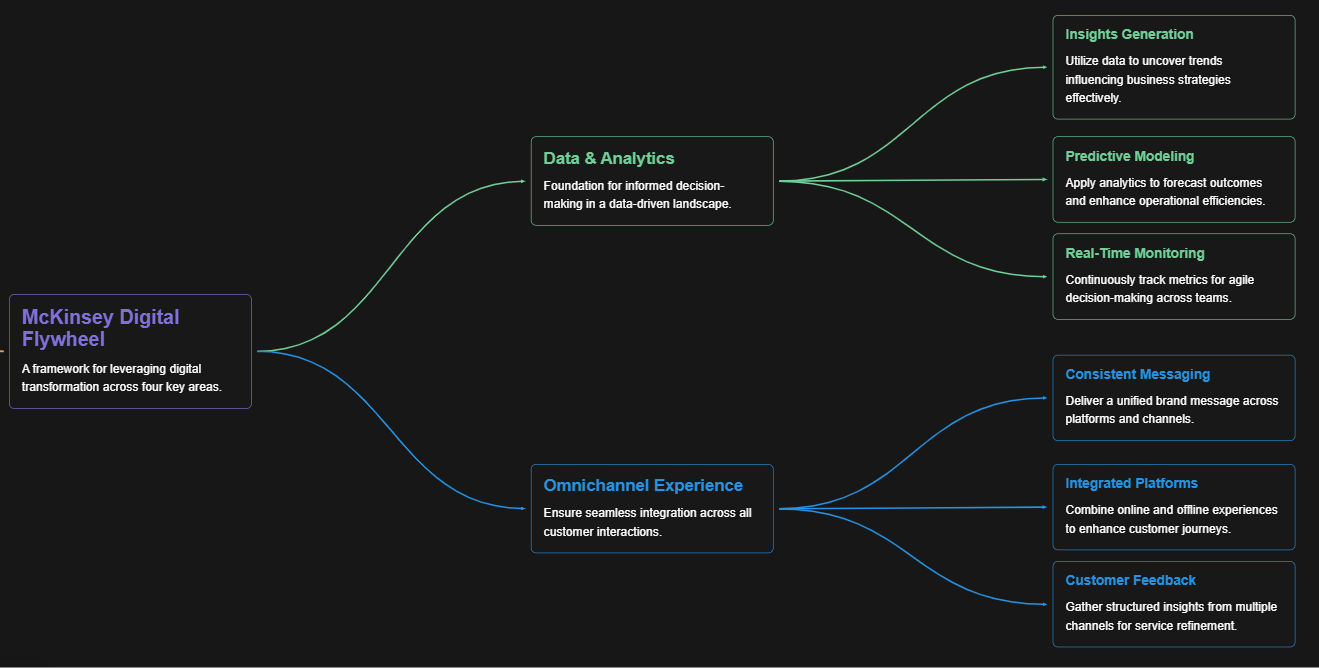
McKinsey Digital Flywheel

McKinsey 9-Box Talent Matrix

McKinsey 7S Framework

The Psychology of Persuasion in Marketing

The Influence of Colors on Branding and Marketing Psychology

What is Marketing?
Recent Blogs

Part 8: From Blocks to Brilliance – How Transformers Became Large Language Models (LLMs) of the series - From Sequences to Sentience: Building Blocks of the Transformer Revolution

Part 7: The Power of Now – Parallel Processing in Transformers of the series - From Sequences to Sentience: Building Blocks of the Transformer Revolution

Part 6: The Eyes of the Model – Self-Attention of the series - From Sequences to Sentience: Building Blocks of the Transformer Revolution

Part 5: The Generator – Transformer Decoders of the series - From Sequences to Sentience: Building Blocks of the Transformer Revolution

Part 4: The Comprehender – Transformer Encoders of the series - From Sequences to Sentience: Building Blocks of the Transformer Revolution of the series - From Sequences to Sentience: Building Blocks of the Transformer Revolution