How Hierarchical Priors Helped Anita Make Smarter, Faster Marketing Decisions
Anita, the head of insights at a fast-growing beauty brand, was running ad campaigns across ten cities. Some cities had loads of historical sales data; others were brand new. The team was struggling: how do you build a model that doesn't get thrown off by patchy data, but still respects local quirks? Their old model treated every city like a separate planet — which led to wild swings in predictions. Another version lumped all cities together, assuming they behaved identically. Both felt wrong. Then her data scientist introduced her to a concept that struck a perfect balance: hierarchical priors. This article details Anita’s journey, explaining what hierarchical priors are, how they work, and why they became indispensable for her team, all while providing a practical example of their implementation.
What Are Hierarchical Priors?
In Bayesian modeling, a prior is a probability distribution that reflects our beliefs about a parameter before observing data. For Anita’s team, their initial models used regular priors, perhaps assuming a fixed average ad effectiveness across all cities. For example, if they were modeling the average ROI of an ad campaign, they might assume it follows a normal distribution, such as N (0.5,0.12), with fixed mean and standard deviation.
However, hierarchical priors take this a step further. Instead of fixing the parameters of the prior, we treat them as random variables with their own priors, called hyperpriors. This creates a multi-level structure that inherently models relationships between groups. For Anita, instead of assuming each city’s ad effectiveness was fixed or entirely independent, her data scientist proposed that each city's effectiveness (βj) would come from a larger, common distribution, around a global average.
Example: Modeling City-Specific Ad Effectiveness
- City-specific ad effectiveness: The effectiveness of an ad campaign in city j, denoted βj, is drawn from a normal distribution. βj∼N(μβ,τβ2) for each city j.
- Hyperpriors: The parameters of this common distribution—the global mean ad effectiveness (μβ) and the variance across city effectiveness values (τβ)—are themselves given priors.
- μβ∼N(0.5,12) (Hyperprior for the global average ad effectiveness)
- τβ∼Half-Cauchy(2) (Hyperprior for the variability of ad effectiveness across cities)
This hierarchy meant that the model could learn both the average ad effectiveness across all regions and each region’s unique response. It was like a "natural fit for nested marketing structures" — each campaign ran across multiple channels, and each channel behaved differently in each region. Hierarchical priors handled this effortlessly, allowing her to model the nested structure without needing to flatten or oversimplify it.
How Hierarchical Priors Work
Anita’s campaigns were complex, involving multiple cities with varying amounts of historical data. The challenge was to avoid "wild swings in predictions" from new cities while not lumping all cities together. Hierarchical priors solved this through a mechanism called partial pooling.
- Partial Pooling Brought the Right Kind of Generalization: "It’s like letting Mumbai teach Nagpur a bit about marketing," her analyst explained. Instead of treating new cities or campaigns as totally unknown, the model would say: "You’re new, yes — but you look a lot like these five others. I’ll start you off there and adjust as I learn more." This meant cities with less data could “borrow strength” from those with more, striking a balance between overfitting noisy signals from small cities and underfitting by ignoring differences. For Anita, even new stores in smaller towns could get decent ROI predictions, informed by the behavior of more mature markets.
- Dynamic Regularization Adjusted Shrinkage Automatically: "This model is like a good editor," Anita quipped. "It quietly fixes our noisy data without making a fuss." With hierarchical priors, regularization (or "shrinkage") happened dynamically. Sparse new data in a new ad channel? The model shrunk estimates toward the mean — a hedge against overreacting. Rich data? The local signal overruled the global trend. This adaptability gave the team more confidence when experimenting with new channels or creatives, knowing the model wouldn’t get whiplash from early results.
- Historical Context Was Enhanced, Not Lost: When integrating new data, traditional setups often meant retraining from scratch. But with hierarchical priors, new insights layered on top of the old. When a new product variant launched with a revised message, the model reused shared ad spend effects from past variants, adjusted for differences in channel mix, and updated global hyperparameters subtly. It was like adding a new chapter to a book — not rewriting the whole novel.
Mathematical Structure of Anita’s Model
Here’s the mathematical structure guiding Anita’s work:
- Hyperpriors (global parameters):
μβ ∼ N(0.5,12) (Global ad effectiveness)
τβ ∼ Half-Cauchy(2) (Variance across regions)
- Region-specific ad effects (parameters):
βj ∼ N(μβ,τβ2) for j=1,…,5 (Ad effect in region j)
- Observed sales (likelihood):
yij∼N(100+ βj⋅xij, 5) (Sales prediction)
Where:
- yij is the observed sales in week i, region j
- xij is ad spend in week i, region j
- βj is the ad effectiveness in region j
"This structure lets the model learn what each region’s ROI is, while still learning the bigger pattern across all regions,” Rishi, Anita's data scientist, explained.
Why Use Hierarchical Priors?
Hierarchical priors offered Anita's team several compelling advantages that transformed their decision-making:
- Smarter Estimates Through Partial Pooling: For Anita, this meant even new stores in smaller towns could get decent ROI predictions, informed by the behavior of more mature markets. Instead of overfitting noisy signals from small cities or underfitting by ignoring differences, partial pooling struck a balance. It gave each region its own estimate — but gently nudged them toward a common-sense middle.
- Makes the Most of Sparse Data: When Anita launched a new product line in Northeast India — a region with little prior campaign history — traditional models balked. But the hierarchical model didn’t panic. It simply looked at similar product lines in similar regions and made its best bet. Instead of saying "We don’t know," it said, "Here’s our best guess — and here’s how confident we are." This dramatically reduced cold-start problems, allowing faster launches in new markets.
- Automatic Regularization That Actually Made Sense: Some ad channels had a lot of data, others barely any. Hierarchical priors automatically applied more “shrinkage” to the noisier channels — gently pulling their estimates toward the overall mean — while letting the stronger ones speak more loudly. This adaptive regularization reduced overfitting and gave her more trust in the insights, especially when reporting back to leadership.
- Less Sensitive to Arbitrary Prior Assumptions: Anita used to spend hours debating what prior to use in their Bayesian models. With hierarchical priors, that stress melted away. Since the hyperparameters (like global ad effectiveness) were learned from the data, the model was more robust and needed less fine-tuning. "It’s like the model adjusts itself as new data rolls in — no constant babysitting required," she said.
How Hierarchical Priors Differ from Regular Priors
To understand the distinction and why Anita's team adopted them, it's helpful to compare hierarchical priors to regular, fixed priors:
- Structure: Regular priors assign fixed distributions to parameters. Hierarchical priors add another layer by treating prior parameters as random variables, creating a multi-level model where each level captures different sources of variation. For Anita, this meant moving beyond simple independent estimates per city to a model where cities were related through shared patterns.
- Information Sharing: Regular priors treat groups independently, with no sharing of information. Hierarchical priors enable partial pooling, allowing groups to influence each other through shared hyperparameters. This meant that while each city’s ad effectiveness was unique, it was informed by the collective experience of all other cities.
- Regularization: Regular priors have fixed regularization. Hierarchical priors, as Anita experienced, adaptively learn the degree of regularization from the data, balancing between group-specific and global estimates. This was the "auto-tuner" that shrank weak signals while letting strong ones breathe.
- Uncertainty: Hierarchical priors model uncertainty not only in the parameters but also in the priors themselves, leading to more comprehensive uncertainty quantification. The biggest shift for Anita wasn't just better predictions — it was better conversations. Instead of debating point estimates, her team now talked in credible intervals. They could say: "In Chennai, there’s a 70% chance Instagram ROI is higher than TV," or "But in Pune, we’re not yet sure — the data’s too thin." This clarity transformed stakeholder confidence.
Practical Example: Modeling Regional Ad Effectiveness with Python
After weeks of planning, Anita’s team was ready to build. Her lead data scientist, Rishi, opened a Jupyter notebook to simulate a real-world media mix problem: regional ad spend versus sales, bringing hierarchical priors to life.
Code Example: Here’s how they simulated the problem and designed the hierarchical model using PyMC
import pymc as pm
import numpy as np
import matplotlib.pyplot as plt

# Simulated data: sales and ad spend for 5 regions
np.random.seed(42)
regions = 5
weeks = 20
true_betas = [0.5, 0.6, 0.7, 0.8, 0.9]  # True ad spend effects per region
ad_spend = [np.random.uniform(100, 1000, weeks) for _ in range(regions)]
sales = [np.random.normal(100 + beta * ad_spend[i], 50, weeks) for i, beta inenumerate(true_betas)]

# Hierarchical model
with pm.Model() as model:
    # Hyperpriors for global ad effect and variance
    mu_beta = pm.Normal('mu_beta', mu=0.5, sigma=1)  # Global ad effect
    tau_beta = pm.HalfCauchy('tau_beta', beta=2)     # Variance across regions

    # Region-specific ad effects
    beta_j = pm.Normal('beta_j', mu=mu_beta, sigma=tau_beta, shape=regions)

    # Likelihood for sales data
    for i in range(regions):
        pm.Normal(f'sales_{i}', mu=100 + beta_j[i] * ad_spend[i], sigma=50, observed=sales[i])

    # Sampling from the posterior
    trace = pm.sample(1000, return_inferencedata=True)
# Plot posterior distributions of ad effects
pm.plot_posterior(trace, var_names=['beta_j'], ref_val=true_betas)
plt.show()
Code Explanation:
- Data Generation: They created a synthetic dataset to test the model logic in a controlled setup. This simulated ad spends and sales for five regions, each with slightly varying true ad effectiveness.
- Model Setup: They defined a mu_beta (global mean ad effect) and tau_beta (shared variance across regions) as hyperpriors. Then, beta_j (region-specific ad effects) were drawn from this shared prior, allowing the model to learn both the average and each region’s unique response.
- Likelihood: Observed sales for each region were modeled using a normal distribution, with the mean determined by base sales plus the region-specific ad effect multiplied by ad spend.
- Sampling and Visualization: Running pm.sample() gave them estimates of each region’s ad effectiveness and the overall shared mean and variance, along with credible intervals. Visualizing with pm.plot_posterior() showed how much each region’s estimate was shrunk toward the global mean, especially when data was noisy. "Region 2 had sparse data, so its effect estimate got pulled toward the group average. Region 5 had strong data — so it stood on its own," Rishi noted.
When Anita’s team added a sixth region or a new channel, they didn’t rebuild the whole model. They simply extended the data, and thanks to the hierarchical setup, the new region’s ad effect was informed by new data, regularized by the global trend, and integrated without retraining from scratch.
Real-World Marketing Wins with Hierarchical Priors
Anita’s story mirrors what many modern marketing teams face. Here’s where hierarchical priors made a clear impact:
- Regional Marketing Optimization: Anita could confidently shift budgets from over-performing cities to underfunded ones with real ROI potential.
- New Market Entry: The team could confidently launch in untapped markets, informed by models that learned from “similar siblings.”
- Budget Allocation by Channel: Every rupee of media spend was backed by a mix of global learnings and local insights, allowing the model to learn, for example, that Instagram works better in Tier 1 cities, while print performs better in smaller towns.
- Deeper Insight Through Better Uncertainty Quantification: Beyond predictions, the clarity of credible intervals transformed stakeholder confidence, enabling bolder, smarter bets.
- Continuous Learning and Integration: The model got smarter with each new signal — like a brain that never stopped evolving, turning data integration from an engineering challenge into a statistical advantage.
Conclusion
Hierarchical priors didn’t just make Anita’s models more accurate; they made her decision-making more confident, her resource allocation smarter, and her conversations more credible. They allowed her team to learn across cities, campaigns, and channels — without losing what made each one unique. This flexible and powerful approach to handling complex, structured data, as demonstrated through Anita's journey and the practical Python example, is a cornerstone of modern Bayesian modeling.
Featured Blogs
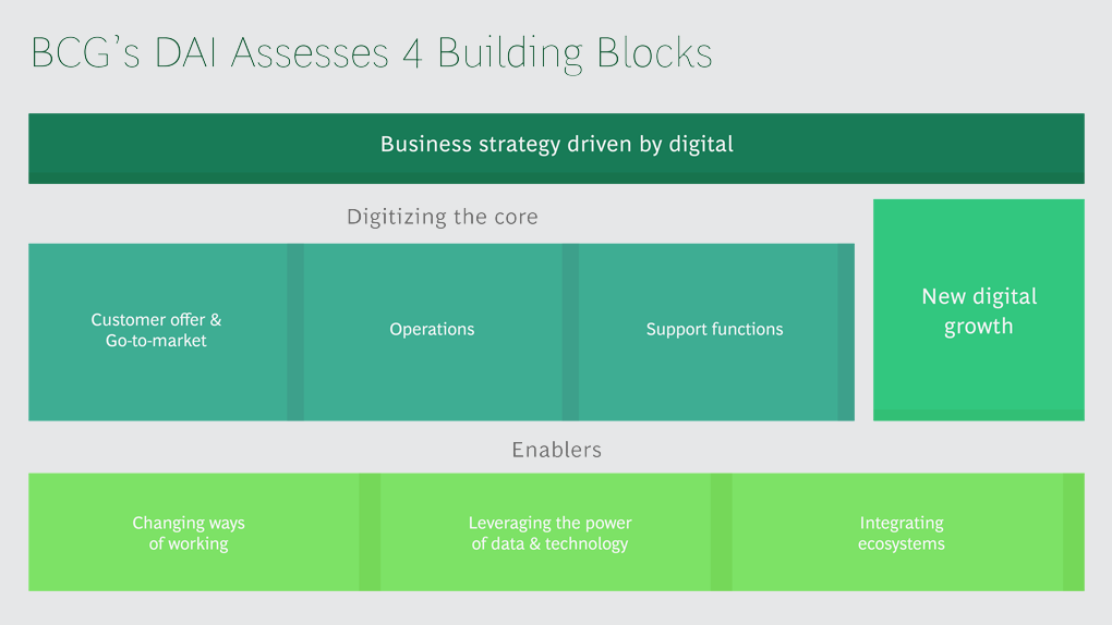
BCG Digital Acceleration Index

Bain’s Elements of Value Framework
McKinsey Growth Pyramid
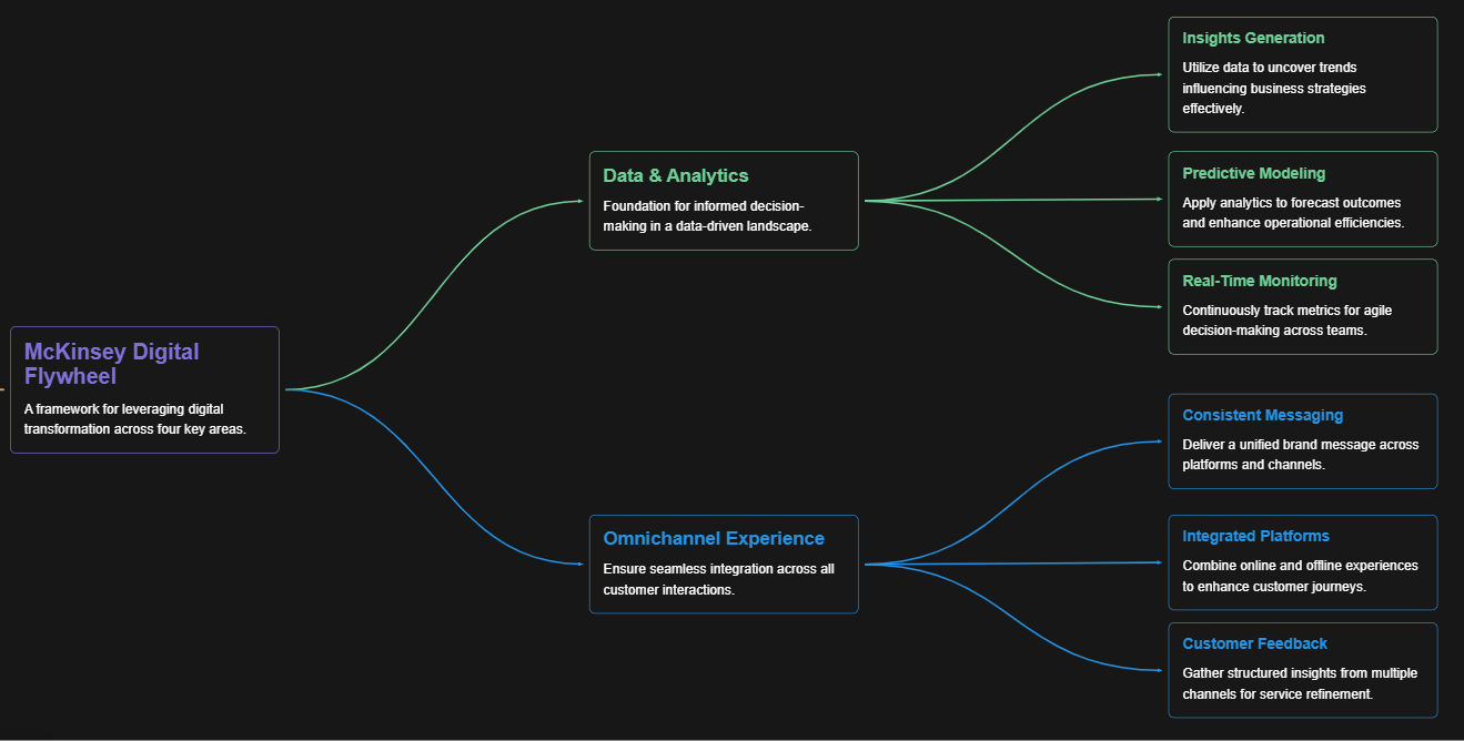
McKinsey Digital Flywheel

McKinsey 9-Box Talent Matrix

McKinsey 7S Framework

The Psychology of Persuasion in Marketing

The Influence of Colors on Branding and Marketing Psychology

What is Marketing?
Recent Blogs

Part 8: From Blocks to Brilliance – How Transformers Became Large Language Models (LLMs) of the series - From Sequences to Sentience: Building Blocks of the Transformer Revolution

Part 7: The Power of Now – Parallel Processing in Transformers of the series - From Sequences to Sentience: Building Blocks of the Transformer Revolution

Part 6: The Eyes of the Model – Self-Attention of the series - From Sequences to Sentience: Building Blocks of the Transformer Revolution

Part 5: The Generator – Transformer Decoders of the series - From Sequences to Sentience: Building Blocks of the Transformer Revolution

Part 4: The Comprehender – Transformer Encoders of the series - From Sequences to Sentience: Building Blocks of the Transformer Revolution of the series - From Sequences to Sentience: Building Blocks of the Transformer Revolution