Non-Parametric Statistics: Methods, Applications & Python Guide

Non-Parametric Statistics

Non-parametric statistics refers to a set of statistical methods that do not assume a specific distribution for the data. These methods are particularly useful when the data does not meet the assumptions required for parametric tests, such as normality or homoscedasticity. Non-parametric methods rely on the rank order of data rather than raw values, making them robust to outliers and applicable to a wide range of datasets.

Table of Contents

• What is a Non-Parametric test?
• Key Characteristics of Non-Parametric Methods
• Common Non-Parametric Tests
• Significance of Non-Parametric Statistics
• Applications of Non-Parametric Methods
• Implementation in Python
• Conclusion

What is a Non-Parametric test?

Non-parametric tests are the mathematical methods used in statistical hypothesis testing, which do not make assumptions about the frequency distribution of variables that are to be evaluated. The non-parametric experiment is used when there are skewed data, and it comprises techniques that do not depend on data pertaining to any particular distribution.

The word non-parametric does not mean that these models do not have any parameters. The fact is, the characteristics and number of parameters are pretty flexible and not predefined. Therefore, these models are called distribution-free models.

Key Characteristics of Non-Parametric Methods

• No Distribution Assumption: Do not require data to follow any specific distribution (e.g., normal distribution).
• Robust to Outliers: Less sensitive to extreme values compared to parametric methods.
• Rank-Based: Analyze data based on order or rank rather than raw values.
• Flexibility: Suitable for ordinal data, small sample sizes, or data with non-linear relationships.

Common Non-Parametric Tests:

Mann-Whitney U Test

The Mann-Whitney U test is a non-parametric statistical test used to determine if there is a difference between the distributions of two independent groups. It is often used when the data does not follow a normal distribution or when the assumption of homogeneity of variances is not met, making it an alternative to the independent samples t-test.

• It does not assume that the data follows a normal distribution.
• While it doesn't directly test means, it compares the ranks of values in the two groups and assesses whether one group tends to have higher or lower values than the other.
• It is used when you have two independent groups (i.e., the samples are not related or paired).

Formula:

where,

• U is the test statistic.
• R is the sum of ranks for one of the groups.
• n is the number of observations in that group.

Assumptions:

• The two samples are independent.
• The data should be at least ordinal (i.e., the values can be ranked).
• The distributions of the two groups do not need to be the same, but the shapes of the distributions are assumed to be similar.

Use Case:

The Mann-Whitney U test is commonly used in cases where you want to compare two groups on a variable, but you cannot assume the data follows a normal distribution. For example, it can be used to compare:

• Treatment vs Control in clinical trials with non-normally distributed outcomes.
• Men vs Women in a survey on opinions or behaviors where responses are not normally distributed.

Wilcoxon Signed-Rank Test

The Wilcoxon Signed-Rank Test is a non-parametric statistical test used to determine if there is a significant difference between the distributions of two related groups. It is often used when the data does not follow a normal distribution and when comparing paired or matched observations, making it an alternative to the paired samples t-test.

• It does not assume that the data follows a normal distribution.
• It compares the differences between paired observations, ranks them, and tests whether the distribution of these differences is centered around zero.
• It is used when you have two related (or paired) groups, meaning the samples are dependent or matched.

Formula:

1. Calculate the differences between paired observations:

 Di  = Xi – Yi  

1. Rank the absolute differences (|Di|), ignoring the signs of the differences.
2. Assign the ranks: For each absolute difference, assign a rank. Ties are given the average of the ranks.
3. Sum the positive and negative ranks:

W+ : Sum of ranks for the positive differences.

W- : Sum of ranks for the negative differences.

1. Test Statistic :  W = min(W+ , W-)
2. Compare the test statistic W to the critical value from the Wilcoxon signed-rank table (based on sample size) to determine significance.

Assumptions:

• The two samples are related or paired (i.e., each data point in one group corresponds to a specific data point in the other group).
• The differences between the paired observations should be at least ordinal (i.e., they can be ranked).
• The distribution of differences should be symmetric (though normality is not required).

Use Case: 

The Wilcoxon Signed-Rank Test is commonly used when comparing two related groups or when the data is ordinal or not normally distributed. For example, it can be used to compare:

• Pre-treatment vs Post-treatment outcomes in clinical trials with non-normally distributed data.
• Before vs After results of an intervention, where the data is paired and the differences between them are not normally distributed.
• Employee satisfaction scores before and after a company policy change.

Kruskal-Wallis Test

The Kruskal-Wallis Test is a non-parametric statistical test used to determine if there are significant differences between the distributions of three or more independent groups. It is often used when the data does not follow a normal distribution or when the assumption of homogeneity of variances is not met, making it an alternative to one-way ANOVA.

• It does not assume that the data follows a normal distribution.
• While it does not directly test means, it compares the ranks of values across the groups and assesses whether one group tends to have higher or lower values than the others.
• It is used when you have three or more independent groups (i.e., the samples are not related or paired).

Formula:

The Kruskal-Wallis test statistic H is calculated using the following formula:

Where:

• N is the total number of observations across all groups.
• k is the number of groups.
• Ri is the sum of ranks for the ith group.
• Ni​ is the number of observations in the ith group.
• ∑ is the summation across all groups.

If the calculated H-statistic is greater than the critical value from the chi-squared distribution (with k−1 degrees of freedom), the null hypothesis that all groups come from the same distribution is rejected, indicating a significant difference between the groups.

Assumptions:

• The samples are independent.
• The data should be at least ordinal (i.e., the values can be ranked).
• The distributions of the groups should be similar in shape, but they do not need to follow the same distribution.

Use Case: 

The Kruskal-Wallis Test is commonly used when comparing three or more independent groups on a variable where the data is ordinal or not normally distributed. For example, it can be used to compare:

• The effectiveness of three different treatments in a clinical trial where the outcomes are not normally distributed.
• Customer satisfaction scores across three or more regions or stores, where the scores are ordinal or skewed.
• Different teaching methods and their impact on student performance in a study with three or more groups.

Spearman's Rank Correlation

Spearman's Rank Correlation is a non-parametric statistical test used to measure the strength and direction of the association between two variables. Unlike Pearson's correlation, which assesses linear relationships, Spearman’s correlation evaluates how well the relationship between two variables can be described using a monotonic function. It is used when the data is ordinal or when the assumptions of Pearson’s correlation (normality, linearity, and homoscedasticity) are not met.

• It does not assume that the data follows a normal distribution.
• It evaluates the relationship by comparing the ranks of values in both variables, rather than their actual values.
• It is used when you have two variables that may not be linearly related but could have a monotonic relationship (i.e., one variable consistently increases or decreases with the other).

Assumptions:

• The data should be at least ordinal (i.e., the values can be ranked).
• The relationship between the variables should be monotonic (i.e., as one variable increases, the other either consistently increases or decreases).
• The paired observations are independent of each other.

Formula:

The Spearman’s rank correlation coefficient ρ\rhoρ (often denoted as rsr_srs​) is calculated using the following formula:

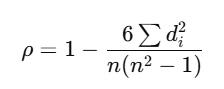
Where:

• di​ is the difference between the ranks of the paired.
• n is the number of paired observations.
• ∑di2​ is the sum of the squared differences of ranks for each pair.

Use Case:

Spearman’s Rank Correlation is commonly used when assessing the relationship between two variables where:

• The variables are ordinal (e.g., ranks, ratings).
• The data is not normally distributed, or when the assumptions for Pearson's correlation are not satisfied.

Chi-Square Test

The Chi-Square Test is a statistical test used to determine if there is a significant association between categorical variables. It is commonly used in contingency table analysis and can assess whether the observed frequencies in different categories significantly differ from the expected frequencies. The test can be used for both goodness of fit (one categorical variable) and independence (two categorical variables).

• It is used when the data is categorical (nominal or ordinal).
• The test compares the observed frequencies of the categories with the expected frequencies under the null hypothesis.
• It is particularly useful in testing relationships between categorical variables.

Types of Chi-Square Tests:

1. Chi-Square Goodness of Fit Test:

• This test is used to determine whether a sample data matches a population with a known distribution.
• It compares the observed frequency distribution to the expected frequency distribution of a categorical variable.

1. Chi-Square Test of Independence:

• This test assesses whether two categorical variables are independent or if there is an association between them.
• It is often used to test hypotheses about the relationship between two variables in a contingency table.

Formula:

The Chi-Square statistic χ2 is calculated using the following formula:

where,

• Oi  is the observed frequency in each category or cell.
• Ei  is the expected frequency in each category or cell.

Assumptions:

• The data should be categorical.
• The observations should be independent of each other.
• Each expected frequency should be at least 5 for the test to be valid.
• The sample size should be sufficiently large (generally n≥30).

Use Case:

The Chi-Square Test is commonly used in situations where you want to determine if there is an association between two categorical variables or if the observed distribution of data fits a specific expected distribution. 

For example,

• Chi-Square Goodness of Fit: To test if a dice is fair (i.e., if the observed distribution of dice rolls matches the expected uniform distribution).
• Chi-Square Test of Independence: To assess if there is an association between gender and voting preference, i.e., if voting behavior is independent of gender.

Significance of Non-Parametric Statistics

• Versatility: Can be applied to a wide range of data types, including ordinal and categorical data.
• Robustness: Performs well even when data violates assumptions of parametric tests.
• Simplified Assumptions: Makes fewer assumptions about the data, increasing applicability.
• Widely Used: Essential in fields such as medical research, social sciences, and market analysis.

Applications of Non-Parametric Methods

• Medical Studies: Comparing treatment effects when data does not follow normal distribution.
• Social Sciences: Analyzing survey data and preferences.
• Environmental Science: Evaluating ecological data with non-linear relationships.
• Market Research: Analyzing customer satisfaction or product rankings.

Implementation in Python

Mann-Whitney U Test

Kruskal-Wallis Test

Spearman's Rank Correlation

Conclusion

Non-parametric statistics provides a versatile and robust toolkit for analyzing data without strict distributional assumptions. These methods are invaluable for real-world datasets that violate the conditions necessary for parametric tests. By utilizing Python libraries such as SciPy, researchers and analysts can efficiently perform non-parametric tests to derive meaningful insights from challenging datasets.