Normal Distribution
Table of Contents
- Introduction to Normal Distribution
- Probability Density Function (PDF) and Cumulative Distribution Function (CDF)
- Importance of Normal Distribution
- Key Characteristics of Normal Distribution
- Practical Applications of Normal Distribution
- Implementing Normal Distribution in Python
- Conclusion
What is Normal Distribution?
The normal distribution, also known as the Gaussian or Laplace-Gauss distribution, is a continuous probability distribution used to describe real-valued random variables. A dataset is considered normally distributed when it follows specific properties associated with the normal distribution.
The normal distribution is mathematically defined by a probability density function (PDF), which determines the likelihood of a continuous random variable occurring within a given range. If f(x)f(x)f(x) represents the probability density function and XXX is a random variable, then the function is integrated over an interval [x,x+dx][x, x + dx][x,x+dx] to determine the probability of XXX falling within that range.
The normal distribution satisfies the following conditions:
f(x) ≥ 0 ∀ x ϵ (−∞,+∞)
And -∞∫+∞ f(x) = 1
Normal Distribution Formula
The probability density function of normal or gaussian distribution is given by;
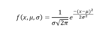
Where,
- x is the variable
- μ is the mean
- σ is the standard deviation
Probability Density Function (PDF) and Cumulative Distribution Function (CDF)
The Probability Density Function (PDF) represents the likelihood of a continuous random variable taking on a specific value. It describes the probability density at different points but does not provide exact probabilities for individual values. Instead, the area under the curve between two points gives the probability of the variable falling within that range.
The Cumulative Distribution Function (CDF), on the other hand, determines the probability that a random variable is less than or equal to a given value. It accumulates probabilities from the leftmost end of the distribution up to a specific point.
Example: Height Distribution
- PDF Interpretation: The PDF may indicate that the probability density of a person being exactly 170 cm tall is higher than at other points.
- CDF Interpretation: The CDF would provide the probability that a person's height is 170 cm or shorter (e.g., 75%).
Visualization:
- The PDF appears as a smooth curve, and the total area under the curve sums to 1.
- The CDF is a monotonically increasing function that starts at 0 and approaches 1 as it moves rightward.
Importance of the Normal Distribution
The normal distribution is fundamental in statistics, probability theory, and numerous scientific disciplines due to its widespread occurrence and essential mathematical properties.
Central Limit Theorem (CLT):
- The CLT states that the sum or average of a sufficiently large number of independent and identically distributed random variables tends to follow a normal distribution, regardless of the original data distribution. This principle is critical in statistical inference and hypothesis testing.
Statistical Methods and Hypothesis Testing:
- Many statistical analyses, including t-tests, ANOVA, and regression, rely on the assumption of normality. This allows for the application of parametric statistical tests that yield meaningful results.
Empirical Rule (68-95-99.7 Rule):
- In a normal distribution:
- 68% of data falls within one standard deviation of the mean.
- 95% of data falls within two standard deviations of the mean.
- 99.7% of data falls within three standard deviations of the mean.
- This rule is useful for understanding data spread and making probabilistic estimates.
- In a normal distribution:
Key Properties of the Normal Distribution
- The mean, median, and mode are all equal.
- The total area under the probability curve is 1.
- The distribution is symmetrical about the mean.
- Exactly half of the data lies to the right and half to the left of the mean.
- The shape of the curve is unimodal, meaning it has only one peak.
- The curve extends infinitely without touching the x-axis.
Real-World Applications of the Normal Distribution
Due to its mathematical properties, the normal distribution is widely used across various domains:
Statistical Analysis & Hypothesis Testing:
- Many inferential statistical techniques assume normality, allowing for confidence interval estimation and hypothesis testing.
Medical Research & Biostatistics:
- Key health parameters like blood pressure, cholesterol levels, and body temperature often follow a normal distribution, aiding in diagnosis and treatment planning.
Quality Control & Manufacturing:
- Ensures product consistency by analyzing variations in production quality. If deviations from normality occur, they may indicate defects.
Finance & Risk Management:
- Financial models use the normal distribution to assess asset returns, stock prices, and risk factors in investment strategies.
Economics & Social Sciences:
- Economic measures like income distribution and demand patterns are often approximated using normal distribution models.
Implementing the Normal Distribution in Python
import numpy as np
import matplotlib.pyplot as plt
from scipy.stats import norm
# Function to plot normal distribution
def plot_normal_distribution(mean, std_dev):
# Generate x values, covering a range around the mean
x_values = np.linspace(mean - 4 * std_dev, mean + 4 * std_dev, 1000)
# Calculate the Probability Density Function (PDF) values
y_values = norm.pdf(x_values, mean, std_dev)
# Plot the normal distribution
plt.figure(figsize=(10, 6))
plt.plot(x_values, y_values, label=f'Normal Distribution\nMean = {mean}, Std Dev = {std_dev}', color='blue')
# Highlight the mean
plt.axvline(mean, color='red', linestyle='--', label='Mean')
# Highlight one standard deviation on either side of the mean
plt.axvline(mean - std_dev, color='green', linestyle='--', label='Mean - 1 Std Dev')
plt.axvline(mean + std_dev, color='green', linestyle='--', label='Mean + 1 Std Dev')
# Title and labels
plt.title('Normal Distribution', fontsize=16)
plt.xlabel('X-axis', fontsize=14)
plt.ylabel('Probability Density Function (PDF)', fontsize=14)
plt.legend(fontsize=12)
plt.grid(True)
plt.show()
# User input for mean and standard deviation
mean = float(input("Enter the mean of the distribution: "))
std_dev = float(input("Enter the standard deviation of the distribution: "))
# Plot the normal distribution based on user input
plot_normal_distribution(mean, std_dev)
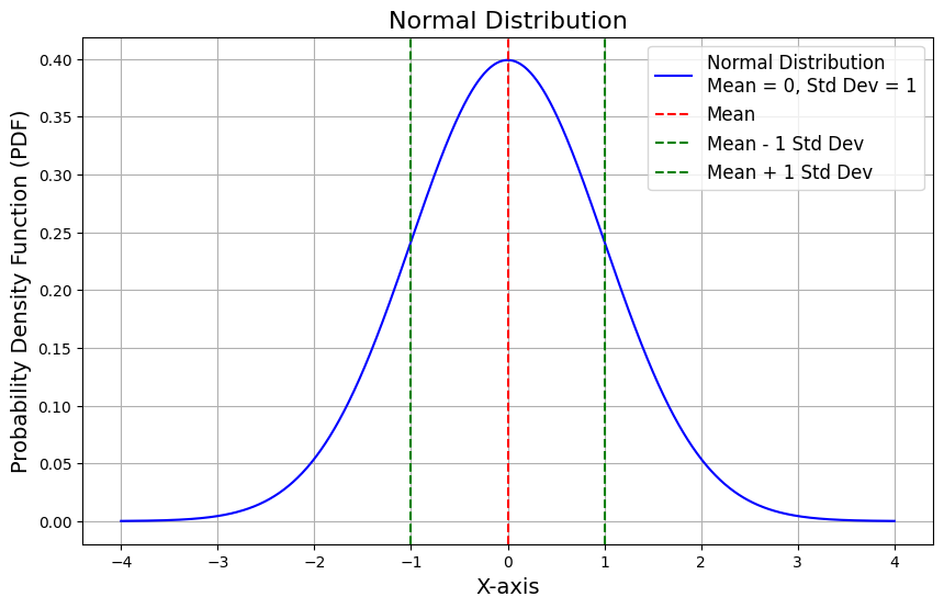
# Plotting the standard normal distribution for comparison
plot_normal_distribution(0, 1)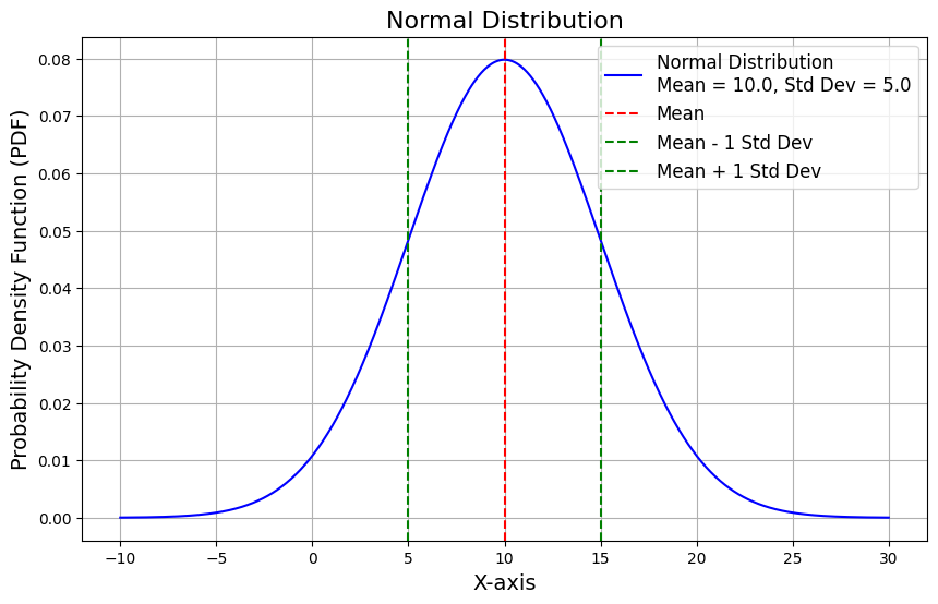
Conclusion
The normal distribution is a fundamental concept in statistics, probability theory, and numerous scientific fields. Its widespread occurrence and mathematical properties make it essential for data analysis and modeling.
Prevalence in Real-World Data:
- Many natural and social phenomena follow a normal distribution, making it a reliable model for diverse applications.
Symmetry and Bell-Shaped Curve:
- The normal distribution has a symmetrical, bell-shaped curve centered around its mean, simplifying statistical calculations and interpretations.
Connection to the Central Limit Theorem (CLT):
- The CLT states that, regardless of the initial distribution, the sum or average of a large number of independent, identically distributed random variables tends to follow a normal distribution. This principle underpins many statistical inference techniques.
Statistical Applications:
- Numerous hypothesis tests and analytical methods, such as t-tests, ANOVA, and regression analysis, assume normality to ensure accurate and meaningful results.
Empirical Rule and Standardization:
- The 68-95-99.7 rule provides a structured way to interpret the spread of data within one, two, or three standard deviations of the mean. Additionally, Z-score standardization allows for comparisons across different datasets following a normal distribution.
Final Thoughts:
The normal distribution serves as a cornerstone in statistical theory and practical applications. Its unique properties make it an invaluable tool for researchers, data analysts, and professionals across various disciplines. A strong understanding of its principles enhances the accuracy and reliability of statistical interpretations, aiding in effective decision-making.
Featured Blogs

BCG Digital Acceleration Index

Bain’s Elements of Value Framework
McKinsey Growth Pyramid
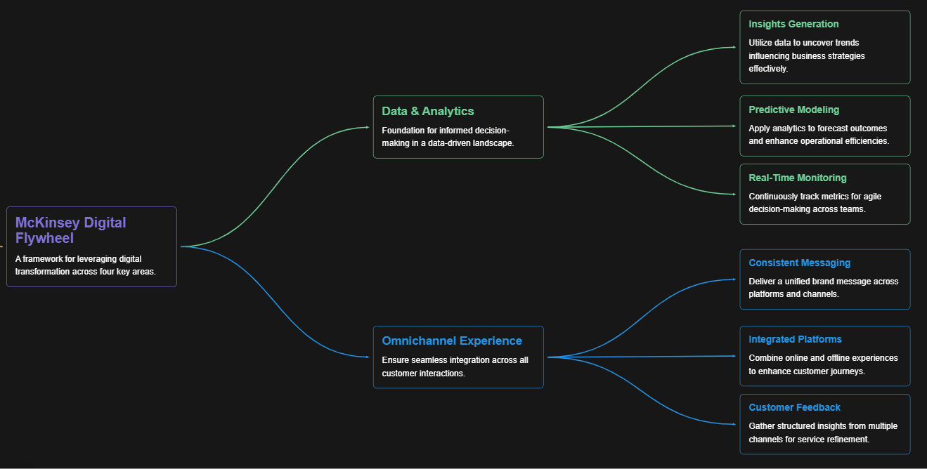
McKinsey Digital Flywheel

McKinsey 9-Box Talent Matrix

McKinsey 7S Framework

The Psychology of Persuasion in Marketing

The Influence of Colors on Branding and Marketing Psychology

What is Marketing?
Recent Blogs

Part 8: From Blocks to Brilliance – How Transformers Became Large Language Models (LLMs) of the series - From Sequences to Sentience: Building Blocks of the Transformer Revolution

Part 7: The Power of Now – Parallel Processing in Transformers of the series - From Sequences to Sentience: Building Blocks of the Transformer Revolution

Part 6: The Eyes of the Model – Self-Attention of the series - From Sequences to Sentience: Building Blocks of the Transformer Revolution

Part 5: The Generator – Transformer Decoders of the series - From Sequences to Sentience: Building Blocks of the Transformer Revolution

Part 4: The Comprehender – Transformer Encoders of the series - From Sequences to Sentience: Building Blocks of the Transformer Revolution of the series - From Sequences to Sentience: Building Blocks of the Transformer Revolution