Key Concepts of Copula
In statistics, a copula is a mathematical function that enables us to understand and model the dependence structure between random variables, separating this structure from their marginal distributions. Essentially, copulas allow us to construct joint probability distributions by combining univariate marginal distributions with a copula that captures the dependence among the variables.
Table of Contents
- Definition and Purpose
- Sklar’s Theorem and Implication
- Uniform marginals
- Types of Dependence
- Copula Families
- Parameter Estimation and Model Selection
- Significance of Copula
- Applications of Copula
- Implementation in Python
- Conclusion
Definition and Purpose
Definition
A copula is a function that links univariate marginal distributions to form a multivariate distribution while preserving their dependency structure. It essentially allows us to construct the joint distribution of random variables when their marginal distributions are known.
Mathematically, a copula C is a function that satisfies:
![]()
where C(u1,u2,...,un) represents the joint cumulative distribution function (CDF) of the transformed uniform variables.
Purpose
The main purpose of copulas is to capture the dependency structure among variables, making it possible to understand and model relationships that are more complex than what simple correlation coefficients can provide.
Sklar’s Theorem and Implication
Theorem
Sklar's theorem is foundational in the theory of copulas. It states that any multivariate joint distribution can be expressed in terms of its marginals and an appropriate copula. For a two-variable case, if F is the joint distribution function with marginals Fx and Fy , then there exists a Copula such that:
![]()
Implication
This theorem implies that copulas enable the separation of marginal behaviour from dependence structure.
Uniform Marginals
In copula theory, uniform marginals refer to the property that the marginal distributions of a copula are always uniformly distributed on the interval [0,1].
Uniform marginals in copula theory provide a standardized way to model dependency structures without being influenced by the original variable distributions. This is a fundamental property that enables the flexibility and power of copulas in multivariate statistical modelling.
Given a set of random variables X1,X2,...,Xn, a copula C allows us to model their joint distribution while separating it from their marginal distributions.
To construct a copula from any given random variables X1,X2,...,Xn , we use the probability integral transform , Ui = Fi(Xi)
Where,
- Fi(Xi) is the cumulative distribution function (CDF) of Xi
- Ui follows a uniform distribution on [0,1], i.e., Ui ∼ U(0,1)
This transformation ensures that the marginal distributions of the copula are always uniform regardless of the original distributions of Xi
Example
Consider two correlated random variables X and Y with marginal distributions Fx and Fy. Their corresponding copula representation uses, U=Fx(X) , V=Fy(Y)
Since U and V uniformly distributed on [0,1], any copula C(U,V) describing their dependence structure will have uniform marginals.
Types of Dependence
In the context of copulas, "dependence" refers to the relationship between random variables that can be modelled beyond simple correlation measures. Copulas are particularly well-suited to capturing different types of dependence structures, including those involving extremal behaviour, which are important in fields such as finance, insurance, and environmental sciences. Here are some key types of dependence that copulas can model:
Linear Dependence: This refers to the traditional type of dependence measured by correlation coefficients. A linear relationship between two variables means that changes in one variable are proportional to changes in another. Gaussian copulas are often used to model linear dependencies.
Non-Linear Dependence: Copulas can model complex, non-linear relationships that aren't captured by linear correlation. Depending on the copula family, these dependencies can take various functional forms.
Positive and Negative Dependence:
- Positive Dependence: Indicates that high values of one variable are associated with high values of another, and vice versa for low values.
- Negative Dependence: High values of one variable are associated with low values of another. Some copulas can represent such anti-extreme behaviour.
4. Tail Dependence:
- Upper Tail Dependence: Describes the tendency of extreme high values of two or more variables to occur together. For instance, if both variables simultaneously reach extreme high values more frequently than would be expected under independence.
- Lower Tail Dependence: Describes the tendency for extreme low values of two or more variables to occur together.
5. Symmetric and Asymmetric Dependence:
- Symmetric Dependence: In a symmetric dependence structure, the relationship between the variables looks the same, regardless of whether we're looking at extreme high or extreme low values, e.g., the Gaussian copula.
- Asymmetric Dependence: The relationship can differ in the tails; one tail may have stronger dependence than the other, seen in copulas like the Clayton or Gumbel.
6. Comonotonicity and Counter monotonicity:
- Comonotonicity: Represents a perfect positive dependence where one variable is an increasing function of another (e.g., moving perfectly together).
- Counter monotonicity: Represents perfect negative dependence, where one variable is a decreasing function of another (e.g., moving perfectly in opposite directions).
7. Exchangeability: This property implies that the joint distribution is invariant to permutations of the random variables, meaning each variable has the same role in the dependence structure.
8. Independence: A copula can also model independence, where the joint distribution is simply the product of the marginal distributions, implying no dependence structure.
Copula Families
Copula families are groups of copulas that share similar mathematical properties and can be used to model different types of dependence structures among random variables. Each family offers unique characteristics and flexibility to capture specific aspects of dependence, such as symmetry, tail dependence, and non-linear relationships. Here are some of the most common copula families:
Gaussian Copula:
- Characteristics: Based on the multivariate normal distribution, the Gaussian copula captures linear dependence structures.
- Features: It does not inherently model tail dependence, meaning it might not be suitable for capturing extreme co-movements.
- Usage: Widely used in finance and risk management due to its simplicity and the straightforward interpretation of its parameters.
2. t-Copula:
- Characteristics: Derived from the multivariate t-distribution, the t-copula can capture both linear dependence and tail dependence.
- Features: The degree of freedom parameter allows the copula to adjust the amount of tail dependence, making it suitable for modeling scenarios with extreme events.
- Usage: Often used in financial contexts where joint extreme events, like simultaneous market crashes, are important.
3. Archimedean Copulas: This family includes several copulas known for their simple, closed-form expressions. They are particularly useful for modeling asymmetric dependencies.
- Clayton Copula: Captures lower tail dependence, making it suitable for modelling risk scenarios where joint low outcomes are crucial.
- Gumbel Copula: Captures upper tail dependence, valuable for situations where joint extreme upper outcomes (like high losses) are of interest.
- Frank Copula: This copula covers a wide range of dependencies, featuring neither upper nor lower tail dependence, thus allowing for modelling moderate dependencies.
4. Extreme Value Copulas:
- Characteristics: These are designed to model extreme events and tail dependencies effectively.
- Types: Examples include the Gumbel copula, which is also an extreme value copula due to its ability to model upper tail dependence.
- Usage: Particularly useful in fields like meteorology and finance, where extreme values are significant.
5. Plackett Copula:
- Characteristics: Can model both positive and negative association but does not exhibit tail dependence.
- Usage: Suitable for scenarios where there is a need to capture mild dependencies without significant extremal behaviour.
6. BB Copulas:
- Characteristics: These are derived from transformations and extensions of basic copulas, like the Clayton or Gumbel, offering more flexibility in capturing varied dependence structures.
- Usage: Used when more flexibility is needed compared to standard copulas.
Each copula family offers different strengths, making them suited for particular types of analyses based on the data's dependence structure. Choosing the right copula family involves understanding the characteristics of the data and the types of dependence that are most critical to capture. In practice, analysts often compare multiple copula models to determine the best fit for their specific applications.
Parameter Estimation and Model Selection
Parameter estimation and model selection are important steps in the application of copulas for statistical modelling. These processes help determine the best-fit copula that describes the dependence structure among variables and estimate the associated parameters.
Parameter estimation
- Method of moments
- Involves matching the empirical moments (e.g., means, variances, covariances) with the theoretical moments derived from the copula model. This method is straightforward but may not always be applicable, especially for complex copulas.
2. Maximum Likelihood Estimation (MLE):
- Process: This is the most common method for estimating copula parameters due to its efficiency and statistical properties. It involves maximizing the likelihood function, which measures the probability of observed data given the parameters.
- Advantages: MLE provides efficient and asymptotically unbiased estimators, particularly for large samples.
- Implementation: Requires numerical optimization techniques, as the likelihood function is usually complex.
3. Inference Function for Margins (IFM):
- Two-Stage Estimation: First, estimate the parameters of the marginal distributions; second, estimate the copula parameters using the pseudo-observations derived from the marginal models.
- Flexibility: Allows separate estimation of marginals and copulas, accommodating different marginal distributions for each variable.
4. Canonical Maximum Likelihood:
- A variant of MLE that focuses on simplifying the estimation procedure by making certain assumptions, particularly useful for high-dimensional data.
5. Pseudolikelihood Methods
- These methods use pseudo-observations (rank-transformed data) to simplify the likelihood function, especially when the sample size is small or the dimensionality is high.
Model Selection
- Goodness-of-Fit Tests:
- Statistical tests assess whether the chosen copula model adequately describes the data. Tests include the Cramér-von Mises or the Anderson-Darling test statistics tailored for copulas.
2. Information Criteria:
- Akaike Information Criterion (AIC) and Bayesian Information Criterion (BIC): These criteria balance model fit with complexity, penalizing the addition of parameters. Lower AIC/BIC values indicate a better model fit relative to complexity.
3. Cross-Validation:
- Divides the data into subsets to validate the copula model's predictive performance and generalizability outside the training sample.
4. Visual Inspection:
- Q-Q Plots and P-P Plots: Compare empirical copula function plots with fitted ones to assess how well the model captures the dependence structure visually.
5. Tail Dependence Analysis:
- Checks whether the copula adequately models the tail dependence structure, particularly for risk management applications where extreme values are of interest.
Significance of Copula
Separation of Marginals and Dependence:
Copulas allow the separate modelling of marginal distributions and the dependence structure, offering greater flexibility and improved accuracy in multivariate modelling. This separation is essential in many applications where different variables may follow different distributions but still exhibit significant interdependencies.
2. Modelling Complex Dependence Structures:
Unlike traditional correlation measures, copulas can capture non-linear dependencies and asymmetries in the relationships between variables. This is crucial for accurately modelling real-world phenomena that involve complex interactions.
3. Tail Dependence:
Copulas can model tail dependence, describing the behaviour of extreme values occurring simultaneously. This capability is vital in risk management. Copulas are significant in various fields due to their ability to model and analyse complex dependencies between random variables, independently of their marginal distributions. This unique capability provides several advantages and applications across different domains
4. Better Risk Management in Finance & Insurance:
Copulas are widely used in finance to model portfolio risk, where asset returns exhibit non-linear dependencies (e.g., stock market crashes). In insurance, copulas help assess the joint likelihood of multiple claims happening together, improving risk assessment models.
5. Flexibility in Constructing Joint Distributions:
Unlike Gaussian distributions, which impose a rigid dependence structure, copulas allow for
- Tail dependence modelling: Capture extreme co-movements of variables.
- Asymmetric dependencies: Model scenarios where variables exhibit different dependence structures in different regions.
6. Simulation and Synthetic Data Generation:
Copulas are useful in Monte Carlo simulations for generating synthetic data that preserves real-world dependencies. This is beneficial in fields like financial stress testing, machine learning data augmentation, and climate modelling.
Applications of Copula
Finance & Risk Management
- Portfolio Risk Modelling: Captures non-linear dependencies for accurate Value-at-Risk (VAR) and risk assessment.
- Credit Risk Analysis: Models joint defaults in collateralized debt obligations (CDOs) and loan portfolios.
- Asset Pricing: Improves pricing of derivatives and options by accounting for tail dependencies.
2. Insurance & Actuarial Science
- Risk Dependency: Models correlated claims in home, auto, and catastrophe insurance.
- Reinsurance Pricing: Helps assess joint claim probabilities for aggregate risk estimation.
3. Machine Learning & Data Science
- Anomaly Detection: Identifies fraud, cyber threats, and outliers in data.
- Synthetic Data Generation: Preserves dependencies for data augmentation.
- Feature Engineering: Transforms correlated features for better predictive modelling.
4. Economics & Social Sciences
- Income & Wealth Distribution: Analyses economic inequality and mobility.
- Consumer Behaviour: Models dependencies in spending patterns.
5. Climate Science & Environmental Studies
- Extreme Weather Events: Predicts joint occurrences of hurricanes, floods, and heatwaves.
- Hydrology & Water Management: Assesses relationships between rainfall, river flow, and dam storage.
6. Medicine & Epidemiology
- Medical Risk Assessment: Models comorbidities and biomarker dependencies.
- Drug Interaction Analysis: Evaluates effects of multiple medications on patients.
7. Engineering & Reliability Analysis
- System Failure modelling: Assesses dependent component failures in power grids, aircraft, and machinery.
- Supply Chain Risk: Models supplier delays and demand fluctuations.
8. Cybersecurity & Network Analysis
- Intrusion Detection: Identifies abnormal patterns in network traffic.
- Fraud Detection: Captures correlations in fraudulent transactions.
Implementation in Python
import numpy as np
from scipy.stats import norm, t, gumbel_r
from copulas.multivariate import GaussianMultivariate

# Define the marginal distributions
dist_x = norm(loc=2, scale=1)  # Normal distribution for X
dist_y = t(df=3, loc=1, scale=2)  # Student's t distribution for Y

# Generate random samples from the marginal distributions
x = dist_x.rvs(size=1000)
y = dist_y.rvs(size=1000)

# Define a Gaussian copula with a correlation of 0.7
copula = GaussianMultivariate(distribution={"copula":  {"name": "gaussian",
                                                       "parameters": {"correlation": [[1.0, 0.7],
                                                                                      [0.7, 1.0]]}}})

# Fit the copula to the data
copula.fit(u=np.array([x, y]).transpose())

# Generate new samples from the joint distribution using the fitted copula
new_samples = copula.sample(num_samples=1000)

# Access the individual variables from the generated samples
new_x = new_samples[:, 0]
new_y = new_samples[:, 1]

# Example of calculating the joint probability using the fitted copula
u = copula.cdf(x=np.array([dist_x.cdf(2.5), dist_y.cdf(0.8)]))
print(f"Joint probability: {u}")
Output:
Joint probability: 0.6921121604392712
Conclusion
Copulas are powerful tools for modelling dependencies between variables, capturing non-linear and tail dependencies beyond traditional correlation measures. They are widely used in finance, insurance, machine learning, and risk management for better risk assessment and predictive modelling.
By separating dependency structure from marginals, copulas offer flexibility in data simulation and analysis. With Python libraries like stats models and SciPy, they can be effectively implemented for real-world applications.
Featured Blogs

BCG Digital Acceleration Index
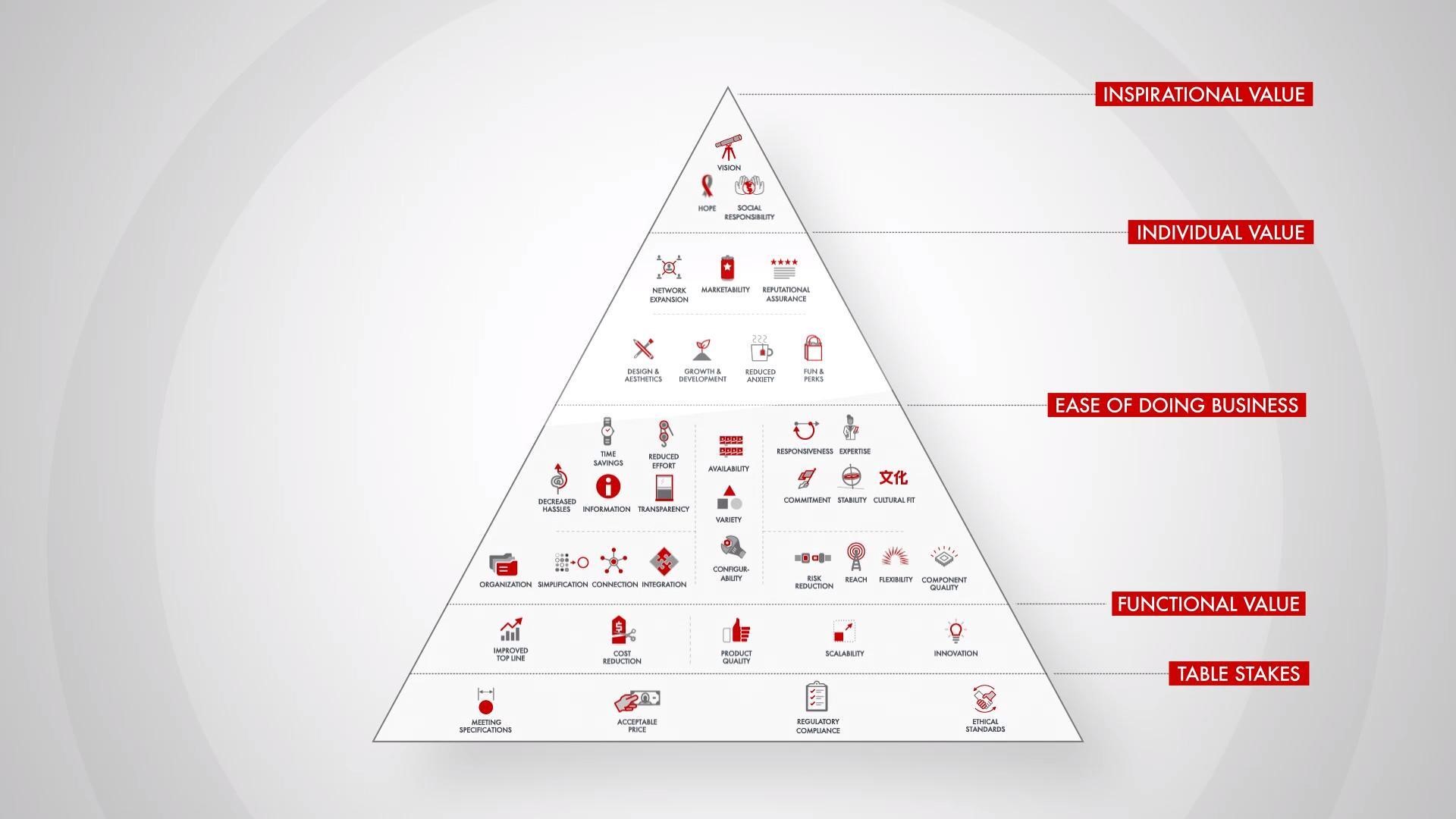
Bain’s Elements of Value Framework
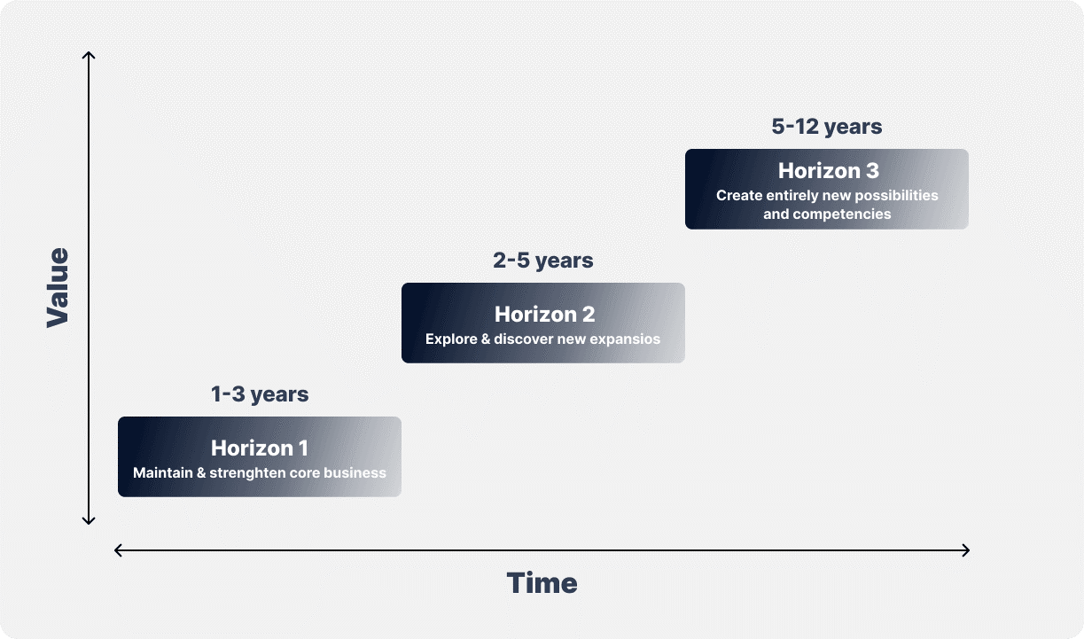
McKinsey Growth Pyramid
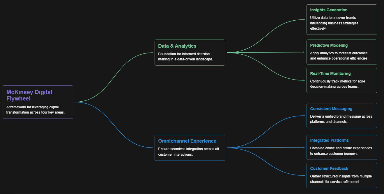
McKinsey Digital Flywheel
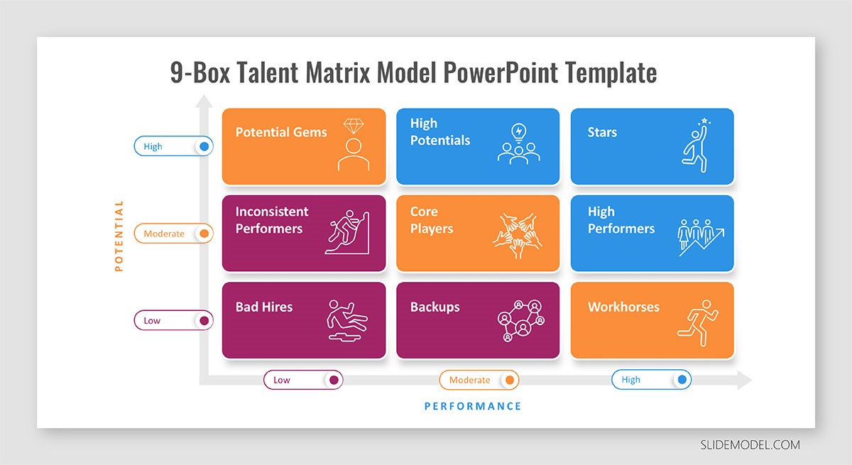
McKinsey 9-Box Talent Matrix

McKinsey 7S Framework
The Psychology of Persuasion in Marketing

The Influence of Colors on Branding and Marketing Psychology

What is Marketing?
Recent Blogs

Part 8: From Blocks to Brilliance – How Transformers Became Large Language Models (LLMs) of the series - From Sequences to Sentience: Building Blocks of the Transformer Revolution

Part 7: The Power of Now – Parallel Processing in Transformers of the series - From Sequences to Sentience: Building Blocks of the Transformer Revolution
Part 6: The Eyes of the Model – Self-Attention of the series - From Sequences to Sentience: Building Blocks of the Transformer Revolution

Part 5: The Generator – Transformer Decoders of the series - From Sequences to Sentience: Building Blocks of the Transformer Revolution

Part 4: The Comprehender – Transformer Encoders of the series - From Sequences to Sentience: Building Blocks of the Transformer Revolution of the series - From Sequences to Sentience: Building Blocks of the Transformer Revolution


