Weibull Probability Density Function
The Weibull distribution is a continuous probability distribution commonly used for analyzing life data, modeling failure times, and assessing product reliability. It is widely applicable across various fields, including engineering, economics, biology, and hydrology. As an extreme value probability distribution, it is frequently employed in reliability analysis, survival studies, wind speed modeling, and other domains.
One of the key advantages of the Weibull distribution is its flexibility—it can effectively represent different types of data by resembling other distributions, such as the normal and exponential distributions. The reliability of a system or product modeled using the Weibull distribution is determined through specific parameters that define its shape and scale.
Types of Weibull Probability Density Functions (PDF):
There are two primary forms of the Weibull probability density function (PDF):
- Two-parameter Weibull PDF
- Three-parameter Weibull PDF
Weibull Distribution Formula:
The general formula for the three-parameter Weibull probability density function (PDF) is:

where:
- K is the shape parameter, determining the distribution's form.
- λ (lambda) is the scale parameter, influencing the spread of the data.
- θ (theta) is the location parameter, shifting the distribution along the x-axis.
The standard Weibull distribution is obtained when the location parameter θ = 0 and the scale parameter λ = 1, simplifying the formula to:
![]()
Two-Parameter Weibull Distribution
The two-parameter Weibull distribution is a simplified version of the three-parameter Weibull distribution, where the location parameter θ is not included. The probability density function (PDF) is given by:

where:
- k is the shape parameter, determining the distribution's form.
- λ (lambda) is the scale parameter, influencing the spread of the data.
- θ (theta) is the location parameter, shifting the distribution along the x-axis.
This distribution is widely used due to its ability to model diverse types of data, making it a fundamental tool in statistical analysis and reliability engineering.
A Weibull plot is a graphical tool used to evaluate whether a dataset follows a two-parameter Weibull distribution with an assumed location parameter of zero. This method helps in visually assessing how well the Weibull distribution fits the given data.
The plot is designed with specialized scales so that if the data aligns with a Weibull distribution, the points will appear in a straight or nearly straight line. By applying a least-squares fit, estimates for the shape (k) and scale (λ) parameters of the Weibull distribution can be obtained.
In this approach:
- The scale parameter (λ) is determined by exponentiating the intercept.
- The shape parameter (k) is calculated as the reciprocal of the slope of the fitted line.
A Weibull probability plot provides a visual way to verify if the distribution accurately describes the dataset, making it a valuable tool in reliability analysis and failure time modeling.

Weibull Distribution Reliability
The Weibull distribution is widely used in reliability analysis and life data analysis due to its flexibility in modeling different types of data. Its ability to adjust to various scenarios makes it an essential tool for assessing failure rates and product durability. The probability density function (PDF) defines the distribution, with parameters that influence the shape, scale, and location of the function. Among various methods available for reliability assessment, the Weibull distribution is one of the most effective for analyzing life data.
Properties of the Weibull Distribution
Key properties of the Weibull distribution include:
- Probability density function (PDF)
- Cumulative distribution function (CDF)
- Moments
- Moment generating function (MGF)
- Shannon entropy
Applications of Weibull Analysis
One of the most common applications of the Weibull distribution is in Weibull analysis, which helps evaluate time-to-failure rates. This analysis is used in various domains, including:
- Warranty analysis
- Manufacturing components (e.g., bearings, capacitors, and dielectric materials)
- Utility services
- Medical and dental implants (evaluating implant longevity)
- Other applications involving time-to-failure modeling
Weibull analysis is useful not only in production stages but also in design and operational phases, ensuring long-term reliability. Today, statistical software programs automate this analysis, making it more accessible and efficient.
Table of Contents
- Introduction to Weibull Distribution
- Applications of the Weibull Probability Density Function (PDF)
- Significance of the Weibull PDF
- Implementation in Python
- Conclusion
Understanding the Weibull Distribution
In certain experiments, a continuous random variable is best represented by a probability distribution that incorporates multiple parameters, providing more flexibility in fitting experimental data. One such distribution is the Weibull distribution, a generalization of the exponential distribution introduced by Waloddi Weibull.
The Weibull distribution is a two-parameter family of curves, initially developed to model material strength. However, its applications have expanded to reliability and lifetime analysis. Unlike the exponential distribution, which assumes a constant failure rate, the Weibull distribution offers greater flexibility by allowing failure rates to vary over time.
Related Distributions
The Weibull distribution is closely associated with several other probability distributions:
Exponential Distribution
- A one-parameter continuous distribution with a mean (μ).
- The Weibull distribution reduces to the exponential distribution when shape parameter (b) = 1, meaning μ = a.
Extreme Value Distribution
- A two-parameter distribution used for modeling the largest or smallest values in a dataset.
- If X follows a Weibull distribution with parameters (a, b), then log(X) follows an extreme value distribution with parameters μ = log(a), σ = 1/b.
- This property is often used to fit data to a Weibull distribution.
Rayleigh Distribution
- A one-parameter continuous distribution used in signal processing and reliability analysis.
- The Rayleigh distribution with scale parameter (b) corresponds to a Weibull distribution with parameters A = √2b and B = 2.

Applications of the Weibull Probability Density Function (PDF)
The Weibull distribution is extensively applied in reliability engineering and survival analysis to model lifetimes of various systems and components. Its shape parameter influences the nature of the distribution, allowing it to resemble an exponential, normal, or other probability distributions, making it highly adaptable.
The Weibull PDF plays a crucial role in modeling time-to-event data across multiple disciplines. Below are some key applications:
Reliability Engineering
- Failure Analysis: Used to determine the lifespan of mechanical and electrical components.
- System Reliability: Helps assess the durability of machines and structures, guiding maintenance and design improvements.
Survival Analysis
- Medical Research: The Weibull distribution models survival times of patients and the time until specific health events occur.
- Medical Device Reliability: Used to estimate failure probabilities of implants and diagnostic equipment.
Quality Control
- Product Lifespan Estimation: Determines the probability of product failures within a given period.
- Manufacturing Defect Prediction: Helps manufacturers evaluate product durability and establish quality assurance protocols.
Importance of the Weibull Probability Density Function (PDF)
The Weibull PDF is widely used across industries because of its ability to model failure rates, survival probabilities, and time-to-event distributions. Below are some of its key contributions:
Reliability Engineering
- Helps predict failure rates of products and components, allowing for proactive maintenance planning.
- Aids in estimating product lifespan, ensuring safety and efficiency in engineering and industrial systems.
Survival Analysis
- Used in healthcare and medical studies to model patient survival rates and estimate disease progression.
- Helps determine the effectiveness of treatments by analyzing survival probabilities over time.
Quality Assurance
- Assists in predicting failure rates in manufactured goods, helping companies refine production standards.
- Enables organizations to design more reliable products and optimize warranty periods based on data-driven insights.
Implementation in Python
import numpy as np
import matplotlib.pyplot as plt
from scipy.stats import weibull_min
def plot_weibull(lambda_param, k_params, x_range):
    """
    Plots Weibull Probability Density Functions for multiple shape parameters.

    Args:
    - lambda_param: Scale parameter (λ) for the Weibull distribution.
    - k_params: List of shape parameters (k) for the Weibull distribution.
    - x_range: Range of x-values to compute the PDF.
    """
    plt.figure(figsize=(10, 6))
    for k_param in k_params:
        weibull_pdf_values = weibull_min.pdf(x_range, c=k_param, scale=lambda_param)
        plt.plot(x_range, weibull_pdf_values, label=f'λ={lambda_param}, k={k_param}')

    plt.title('Weibull Probability Density Function (PDF)')
    plt.xlabel('x')
    plt.ylabel('PDF')
    plt.legend(title="Weibull PDFs", loc="best")
    plt.grid(True)
    plt.show()

# Define scale parameter and a list of shape parameters
lambda_param = 10  # Scale parameter (λ)
k_params = [0.5, 1, 2, 4]  # Different shape parameters (k)
x_values = np.linspace(0, 30, 500)  # x-values from 0 to 30

# Plot the Weibull PDFs for the specified shape parameters
plot_weibull(lambda_param, k_params, x_values)

def plot_weibull_scale_comparison(k_param, lambda_params, x_range):
    """
    Plots Weibull Probability Density Functions for multiple scale parameters.

    Args:
    - k_param: Shape parameter (k) for the Weibull distribution.
    - lambda_params: List of scale parameters (λ) for the Weibull distribution.
    - x_range: Range of x-values to compute the PDF.
    """
    plt.figure(figsize=(10, 6))
    for lambda_param in lambda_params:
        weibull_pdf_values = weibull_min.pdf(x_range, c=k_param, scale=lambda_param)
        plt.plot(x_range, weibull_pdf_values, label=f'λ={lambda_param}, k={k_param}')

    plt.title('Weibull PDF with Different Scale Parameters (k constant)')
    plt.xlabel('x')
    plt.ylabel('PDF')
    plt.legend(title="Weibull PDFs", loc="best")
    plt.grid(True)
    plt.show()

# Define shape parameter and a list of scale parameters
k_param = 2  # Shape parameter (k)
lambda_params = [5, 10, 15]  # Different scale parameters (λ)

# Plot the Weibull PDFs for the specified scale parameters
plot_weibull_scale_comparison(k_param, lambda_params, x_values)

Conclusion
To summarize, the Weibull Probability Density Function (PDF) is a highly adaptable statistical tool with widespread applications across multiple industries. Its importance stems from its ability to effectively represent lifetimes, durations, and time-to-event data, offering valuable insights into reliability, survival analysis, and risk assessment in various fields.
Featured Blogs

BCG Digital Acceleration Index

Bain’s Elements of Value Framework
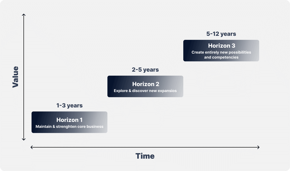
McKinsey Growth Pyramid
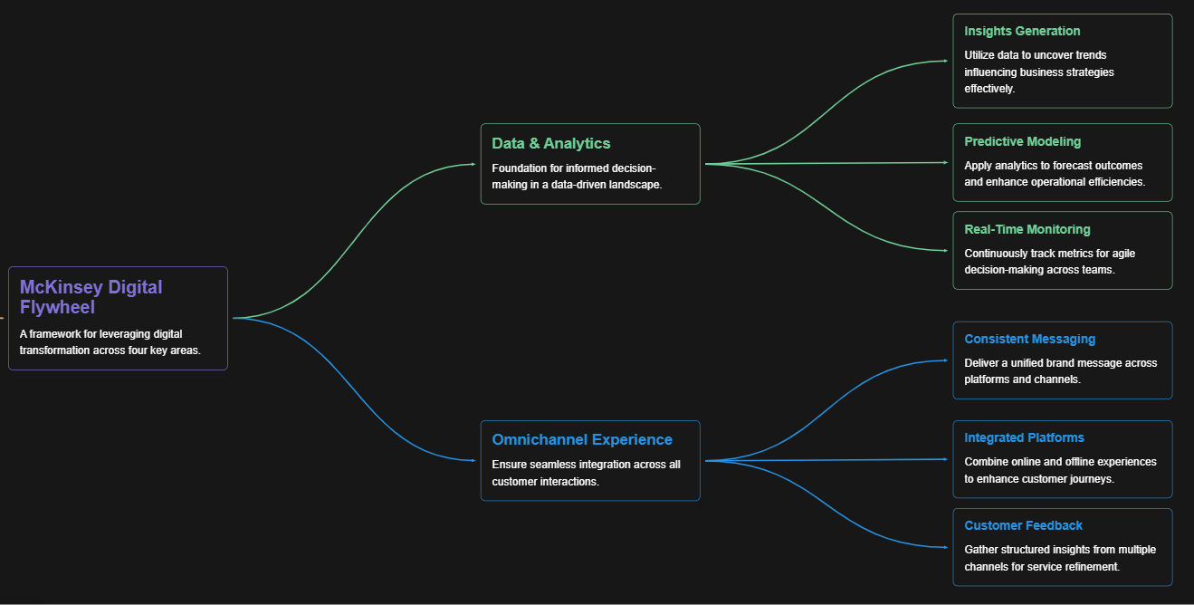
McKinsey Digital Flywheel

McKinsey 9-Box Talent Matrix

McKinsey 7S Framework

The Psychology of Persuasion in Marketing

The Influence of Colors on Branding and Marketing Psychology

What is Marketing?
Recent Blogs

Part 8: From Blocks to Brilliance – How Transformers Became Large Language Models (LLMs) of the series - From Sequences to Sentience: Building Blocks of the Transformer Revolution

Part 7: The Power of Now – Parallel Processing in Transformers of the series - From Sequences to Sentience: Building Blocks of the Transformer Revolution
Part 6: The Eyes of the Model – Self-Attention of the series - From Sequences to Sentience: Building Blocks of the Transformer Revolution

Part 5: The Generator – Transformer Decoders of the series - From Sequences to Sentience: Building Blocks of the Transformer Revolution

Part 4: The Comprehender – Transformer Encoders of the series - From Sequences to Sentience: Building Blocks of the Transformer Revolution of the series - From Sequences to Sentience: Building Blocks of the Transformer Revolution