Types of Copulas
Copulas are mathematical functions that describe the dependency between random variables. They provide a way to model the joint distribution of multiple variables while preserving their individual marginal distributions. Copulas are widely used in fields like finance, risk management, and statistics for modelling dependencies that are not captured by linear correlation alone.
Table of Contents
- Introduction to Copulas
- Gaussina Copula
- Definition and Structure
- Characteristics
- Applications
- Limitations
- Implementation in Python
3. Clayton Copula
- Definition and Structure
- Characteristics
- Applications
- Limitations
- Implementation in Python
4. Gumber Copula
- Definition and Structure
- Characteristics
- Applications
- Limitations
- Implementation in Python
5. Frank Copula
- Definition and Structure
- Characteristics
- Applications
- Limitations
- Implementation in Python
6. Student-t Copula
- Definition and Structure
- Characteristics
- Applications
- Limitations
- Implementation in Python
Introduction to Copulas
A copula is a function that links the marginal distributions of multiple variables to their joint distribution. It allows us to separate the dependency structure from the marginal distributions, making it a powerful tool in multivariate analysis.
The concept of copulas originates from probability theory and has been extensively used in statistics and finance. Traditional correlation measures such as Pearson’s correlation only capture linear relationships, whereas copulas can model complex, nonlinear dependencies, including tail dependencies. This makes them highly valuable in risk management, as they allow analysts to better understand extreme events and co-movements in financial markets. Copulas also enable the construction of joint distributions from arbitrary marginal distributions, providing flexibility in statistical modelling.
Types of Copulas
Different types of copulas exist based on their dependency structures:
Gaussina Copula
A Gaussian copula is a statistical tool used to model and analyse the dependence structure between multiple variables, especially in finance, risk management, and machine learning. It allows the modelling of complex dependencies using a multivariate normal distribution while maintaining the flexibility to use different marginal distributions for individual variables.
Definition and Structure
The Gaussian copula is constructed by transforming the standard normal marginal distributions into uniform marginals using the cumulative distribution function (CDF). The copula function combines these marginals to form a multivariate distribution.
Mathematical Formulation:
- Assume Z1,Z2,…,Zn are standard normal variables with a correlation matrix Σ.
- The Gaussian copula functions by mapping each Zi through the standard normal CDF to get uniform variables Ui=Φ(Zi).
- The copula C for random variables X1,X2,…,Xn with marginals F1,F2,…,Fn is given by:
![]()
where Φ−1 is the inverse CDF of the standard normal distribution and ΦΣ is the CDF of the multivariate normal distribution with correlation matrix Σ.
Characteristics
- Linear Dependence: The Gaussian copula captures linear correlations between variables as specified by the correlation matrix ΣΣ, but does not model tail dependence, meaning it might not be ideal for scenarios where joint extreme events are critical.
- Symmetry: The Gaussian copula is symmetric, meaning it treats both tails of the distribution equally.
- Flexibility with Marginals: While the Gaussian copula itself models normal variables, it can be used with any marginal distribution, making it suitable for various types of data.
Applications
- Finance and Risk Management: In credit risk modelling, the Gaussian copula can simulate the joint default probability of different obligors (e.g., companies defaulting on debts). It underlies many models for pricing and managing portfolios of correlated assets.
- Dependence Modelling: In scenarios where the primary concern is capturing linear relationships without extremal dependencies, the Gaussian copula is a suitable choice.
Limitations
- Lack of Tail Dependence: Although effective for capturing linear dependencies, the Gaussian copula does not model tail dependence, limiting its use in situations that involve the co-movement of extreme values, such as systemic risk in finance.
Implementation in Python
          import numpy as np
          from scipy.stats import norm, multivariate_normal

          # Define the correlation matrix for 2 variables
          correlation_matrix = np.array([[1, 0.7], [0.7, 1]])

          # Create a Gaussian copula with the specified correlation
          def gaussian_copula(u, rho):
           norm_inv = norm.ppf(u)  # Inverse CDF (quantile function)
           return multivariate_normal.cdf(norm_inv, cov=rho)

          # Example usage with two-dimensional uniform inputs
          u = [0.5, 0.5]
          copula_value = gaussian_copula(u, correlation_matrix)
          print("Gaussian copula value:", copula_value)
2. Clayton Copula
The Clayton copula is a popular member of the Archimedean family of copulas, known for capturing dependencies with asymmetry, particularly emphasizing lower tail dependence. It is widely used in fields where the joint behaviour of variables when they take extreme low values is of interest, such as in credit risk and insurance.
Definition and Structure
- Generator Function: The Clayton copula is defined using a generator function, a core characteristic of Archimedean copulas. The generator ψ(t) for the Clayton copula is:
![]()
where θ>0 is the copula parameter controlling the strength of dependence.
- Copula Function: For a two-dimensional case, the copula function for random variables U and V with uniform marginals is defined as:
![]()
Where,
θ: Controls the degree of dependence.
If θ=0, the variables are independent.
As θ increases, the dependence becomes stronger.
Characteristics
- Lower Tail Dependence: The Clayton copula is particularly known for its ability to model lower tail dependence, where it is likely that both variables simultaneously realize low values more frequently than would be expected under independence.
- Asymmetry: Unlike symmetric copulas like the Gaussian, the Clayton copula models an asymmetric dependence structure, which is essential in applications where lower tail dependence is significant.
- Simple Functional Form: The Clayton copula has a relatively simple analytical form, making it easier to work with in many applications.
Applications
- Insurance and Risk Management: Used to model the joint behaviour of risks, especially where extreme losses (lower tails) need to be closely examined, such as simultaneous claims in insurance portfolios.
- Finance: Can be applied to assess credit risk where the primary concern might be the joint default probabilities that occur under adverse conditions.
- Hydrology and Environmental Sciences: Useful in modelling joint low-flow events in rivers, where such behaviour is critical for understanding potential drought conditions or the impact of climate change.
Limitations
- Upper Tail Dependence: While effective in modelling lower tail dependence, the Clayton copula does not capture upper tail dependence, which limits its use in situations where extreme upper values are of interest.
Implementation in Python
import numpy as np

# Clayton copula function for two variables
def clayton_copula(u, v, theta):
                     if theta <= 0:
raise ValueError("Theta must be greater than 0 for Clayton copula.")
                    result = (u**(-theta) + v**(-theta) - 1)**(-1/theta)
                    return result

# Example usage
u = 0.5  # First variable with uniform distribution
v = 0.3  # Second variable with uniform distribution
theta = 2.0  # Dependence parameter

copula_value = clayton_copula(u, v, theta)
print("Clayton copula value:", copula_value)
3. Gumbel Copula
The Gumbel copula is a well-known member of the Archimedean family of copulas and is particularly effective at capturing asymmetric dependencies, specifically in the upper tails. This makes it suitable for modeling scenarios where joint extreme upper values (e.g., joint high losses or extreme events) tend to occur more frequently.
Definition and Structure
The Gumbel copula is defined by a single parameter θθ, which governs the strength of the dependence:

Parameter θ:
- θ≥1: The parameter controls the level of dependence. As θ approaches 1, the copula approaches independence. As θ increases, the dependence becomes stronger, particularly in the upper tail.
- The Gumbel copula parameter θ cannot be less than 1.
Characteristics
- Upper Tail Dependence: The Gumbel copula is particularly known for modelling upper tail dependence, meaning it effectively captures scenarios where extreme high values of variables occur together.
- Asymmetry: The copula exhibits an asymmetric structure, which is beneficial for applications where joint upper tail behaviour is crucial.
- Dependence Structure: It captures dependencies effectively using a relatively simple mathematical form, with stronger dependence as θ increases.
Applications
- Risk Management and Finance: Used in financial modelling and risk assessments where joint extreme positive movements in asset returns or market variables are significant concerns (e.g., correlated defaults).
- Environmental Sciences: Applied in modelling joint occurrences of extreme weather events, such as heavy rainfall or high temperatures, where simultaneous extreme values are critical.
- Insurance: Useful for analysing risks associated with rare but impactful events, such as large claims occurring at the same time.
Limitations
- Lower Tail Dependence: While the Gumbel copula excels at modelling upper tail dependence, it does not capture lower tail dependencies. Thus, it may not be suitable for scenarios where joint low values are significant.
Implementation in Python
import numpy as np

# Gumbel copula function for two variables
def gumbel_copula(u, v, theta):
                   if theta < 1:
                     raise ValueError("Theta must be greater or equal to 1 for Gumbel copula.")
          part1 = (-np.log(u))**theta
          part2 = (-np.log(v))**theta
           result = np.exp(-((part1 + part2)**(1/theta)))
          return result

# Example usage
u = 0.5  # First variable with uniform distribution
v = 0.5  # Second variable with uniform distribution
theta = 2.0  # Dependence parameter

copula_value = gumbel_copula(u, v, theta)
print("Gumbel copula value:", copula_value)
4. Frank Copula
The Frank copula is another member of the Archimedean family of copulas, characterized by its ability to model symmetric dependencies without the Frank copula is another member of the Archimedean family, known for its ability to model both positive and negative dependencies symmetrically. It is particularly flexible because it can handle a wide range of dependence structures without expressing tail dependence, unlike other Archimedean copulas like Clayton or Gumbel.
Definition and Structure
The Frank copula is parameterized by a single parameter θ, which governs the strength and direction of dependence between the variables. It is defined as:

Parameter θ:
- θ=0: This represents independence between variables.
- θ>0: Indicates positive dependence between the variables.
- θ<0: Represents negative dependence.
- θ varies over the entire real line, excluding zero, offering symmetry in treating positive and negative dependencies.
Characteristics
- Symmetric Dependence: Unlike the Clayton and Gumbel copulas, the Frank copula is symmetric; it treats both tails of the distribution similarly, meaning it neither Favors upper nor lower tail dependence.
- Flexibility: It can model a wide range of dependence structures due to its parameter flexibility, accommodating cases with varying degrees of correlation.
- Lack of Tail Dependence: The Frank copula is not specifically tailored for modelling joint extreme events in either tail.
Applications
- Finance and Economics: Used in scenarios where moderate dependencies without extreme joint tail behaviour are needed to be modelled, such as the dependence structure of return series.
- Biostatistics and Epidemiology: Helpful in analysing data where the focus is on average or moderate relationships rather than extreme co-movements.
- Environmental Sciences: Applied to study environmental factors where symmetric, moderate dependencies exist, without strong concerns about joint extremes.
Limitations
- No Tail Dependence: If an analysis requires modelling the occurrence of extreme joint events, the Frank copula may not be suitable due to its lack of tail dependence.
Implementation in Python
import numpy as np

# Frank copula function for two variables
def frank_copula(u, v, theta):
                    if theta == 0:
                      raise ValueError("Theta cannot be zero for the Frank copula.")

           e_theta_u = np.exp(-theta * u)
          e_theta_v = np.exp(-theta * v)
          numerator = (e_theta_u - 1) * (e_theta_v - 1)
          denominator = np.exp(-theta) - 1
          result = -1/theta * np.log(1 + numerator / denominator)
          return result

# Example usage
u = 0.5  # First variable with uniform distribution
v = 0.3  # Second variable with uniform distribution
theta = 2.0  # Dependence parameter

copula_value = frank_copula(u, v, theta)
print("Frank copula value:", copula_value)
5. Student-t Copula
The Student-t copula, often referred to as the t-copula, is a popular choice for modelling dependencies that goes beyond linear correlation, especially in finance and risk management. It derives from the multivariate Student's t-distribution and is valued for its ability to capture both linear dependencies and symmetric tail dependencies (The Student-t copula is a type of copula derived from the multivariate Student-t distribution. It is particularly useful in modelling dependencies where both linear correlation and tail dependence are important. The ability of the Student-t copula to model joint extreme outcomes makes it valuable in fields like finance and risk management.
Definition and Structure
- Parameterization: The Student-t copula is characterized by two main parameters:
- Correlation Matrix (Σ): Similar to the correlation matrix used in the Gaussian copula, it defines the linear relationships between the variables.
- Degrees of Freedom (ν): This parameter captures the tail heaviness. Lower degrees of freedom indicate heavier tails, meaning greater probability of joint extremes.
- Copula Function:
- If T1,ν indicates the univariate Student-t distribution with ν degrees of freedom, and Td,ν,Σ represents the multivariate Student-t distribution with correlation matrix Σ, the Student-t copula for variables with marginal distributions transformed to t-distributions is:
![]()
Here, Tν−1 is the quantile function (inverse CDF) of the univariate Student-t distribution.
Characteristics
- Tail Dependence: Unlike the Gaussian copula, the Student-t copula can capture both upper and lower tail dependence, making it suitable for modelling co-movements of extreme values.
- Symmetry: It provides a symmetric representation of dependencies, treating both tails equally.
- Flexibility: The degrees of freedom parameter allows the model to adjust the heaviness of the tails, providing flexibility in capturing the extremal behavior of the data.
Applications
- Finance and Risk Management: Commonly used for modelling the joint distribution of asset returns where the risk of joint extreme losses or gains is significant. This includes portfolio risk management and credit risk modelling.
- Insurance: Used to assess risks of joint extreme claims where heavy-tailed behaviour is observed.
- Environmental Sciences: Applied in scenarios involving extreme weather events or natural phenomena where the extremal dependency structure is crucial.
Limitations
- Complex Estimation: Given its reliance on both a correlation matrix and degrees of freedom, parameter estimation can be computationally intensive, especially for high-dimensional data.
Implementation in Python
import numpy as np
from scipy.stats import t, multivariate_normal

# Parameters
nu = 4  # Degrees of freedom
corr_matrix = np.array([[1, 0.5], [0.5, 1]])  # Correlation matrix

# Define inverse of the univariate t-distribution for given DOF
def t_inv(u, nu):
    return t.ppf(u, nu)

# Multivariate t-cdf function using scipy's multivariate normal approximation
def student_t_copula(u, nu, corr_matrix):
    # Transform uniform marginals to t marginals
    t_marginals = [t_inv(ui, nu) for ui in u]
              # Compute cdf under multivariate t distribution
    mean = np.zeros(len(u))
    return multivariate_normal.cdf(t_marginals, mean=mean, cov=corr_matrix)

# Example usage
u = [0.5, 0.5]
copula_value = student_t_copula(u, nu, corr_matrix)
print("Student-t copula value:", copula_value)Featured Blogs

BCG Digital Acceleration Index

Bain’s Elements of Value Framework
McKinsey Growth Pyramid
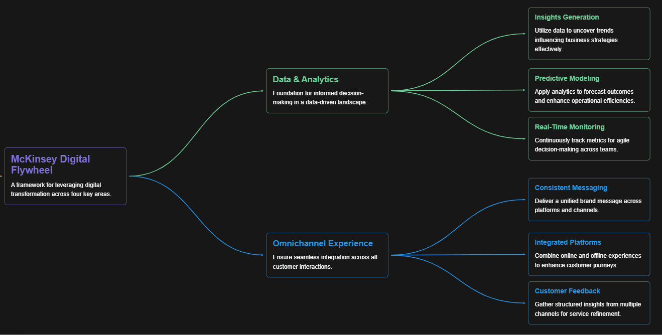
McKinsey Digital Flywheel

McKinsey 9-Box Talent Matrix

McKinsey 7S Framework

The Psychology of Persuasion in Marketing

The Influence of Colors on Branding and Marketing Psychology

What is Marketing?
Recent Blogs

Part 8: From Blocks to Brilliance – How Transformers Became Large Language Models (LLMs) of the series - From Sequences to Sentience: Building Blocks of the Transformer Revolution

Part 7: The Power of Now – Parallel Processing in Transformers of the series - From Sequences to Sentience: Building Blocks of the Transformer Revolution

Part 6: The Eyes of the Model – Self-Attention of the series - From Sequences to Sentience: Building Blocks of the Transformer Revolution

Part 5: The Generator – Transformer Decoders of the series - From Sequences to Sentience: Building Blocks of the Transformer Revolution

Part 4: The Comprehender – Transformer Encoders of the series - From Sequences to Sentience: Building Blocks of the Transformer Revolution of the series - From Sequences to Sentience: Building Blocks of the Transformer Revolution