Bernoulli Distribution
The Bernoulli distribution is a discrete probability distribution used to model experiments that have only two possible outcomes—typically represented as success (1) or failure (0). The probability of success is denoted by ppp, while the probability of failure is 1−p1 - p1−p. Any trial that follows this pattern is referred to as a Bernoulli trial. A simple example of this distribution is passing or failing an exam.
Table of Contents
- Introduction to Bernoulli Distribution
- Importance of Bernoulli Distribution
- Practical Applications
- Implementing Bernoulli Distribution in Python
- Conclusion
Introduction to Bernoulli Distribution
The Bernoulli distribution is a fundamental discrete probability distribution that describes a process in which a single experiment yields one of two outcomes: success or failure. It is a special case of the Binomial distribution where only one trial is conducted.
This distribution is frequently used to model events with binary outcomes. The Swiss mathematician Jacob Bernoulli introduced this concept, which has since become an essential tool in probability and statistics.
If a Bernoulli trial results in a value of 1, it signifies success with a probability of ppp. Conversely, a value of 0 indicates failure, which occurs with a probability of 1−p1 - p1−p.
In Python, the NumPy library provides functions to compute values for a Bernoulli distribution. By plotting histograms, we can visualize the probability distribution of a Bernoulli variable.
Example of Bernoulli Distribution
Consider a scenario where a fair coin is flipped. If heads appear, we consider it a success. Since the probability of getting heads is p=1/2p = 1/2p=1/2, we can define a random variable XXX that follows a Bernoulli distribution:
![]()
Mathematical Representation
A Bernoulli-distributed random variable XXX is also known as an indicator variable since it signals whether an event occurs (1) or not (0). The notation for this distribution is:
![]()
Probability Mass Function (PMF)
The probability mass function (PMF) defines the likelihood of a discrete random variable taking a specific value. For a Bernoulli random variable XXX, the PMF is expressed as:
F(x)=0 x<0
F(x)=1-p 0≤x<1
F(x)=1 x≥1
This function provides a cumulative probability measure, summing up the likelihood of all possible outcomes up to a specified value.
The cumulative distribution function (CDF) of a Bernoulli random variable XXX gives the probability that XXX is less than or equal to a specific value xxx. It is mathematically defined as:![]()
![]()
![]()
![]()
Mean and Variance of the Bernoulli Distribution
The mean, also known as the expected value, of a Bernoulli-distributed random variable is given by:
E[X]=p
The variance of the distribution measures the spread of the values and is determined by the difference between the expected value of X2X^2X2 and the square of the mean. Mathematically, this is represented as:
Var[X]=E[X2]−(E[X])2
For a Bernoulli distribution, the variance simplifies to:
Var[X]=p(1−p)=p⋅q
where q=1−pq = 1 - pq=1−p.
Graphical Representation of the Bernoulli Distribution
A Bernoulli distribution can be visualized using a probability mass function (PMF) graph. This graph provides a clear depiction of the probabilities associated with the two possible outcomes (success and failure) of a Bernoulli random variable.

A graphical representation of the Bernoulli distribution illustrates the probability of success (ppp) when X=1X = 1X=1 and the probability of failure (1−p1 - p1−p, also denoted as qqq) when X=0X = 0X=0. This visualization helps in understanding the probability mass function (PMF) of a Bernoulli random variable.
Importance of the Bernoulli Distribution
The Bernoulli distribution plays a crucial role in various fields due to its ability to model events with binary outcomes. Below are key reasons why it is significant:
- Modeling Binary Outcomes: The Bernoulli distribution is specifically designed for events with only two possible results, such as success/failure or heads/tails. It is widely used in statistical analysis where binary decision-making is involved.
- Foundation for the Binomial Distribution: This distribution serves as the building block for the binomial distribution, which extends the Bernoulli concept to multiple independent trials, allowing the study of repeated binary events.
- Straightforward Probability Model: The Bernoulli distribution provides a simple yet effective way to model probability in binary scenarios. Its single parameter (ppp, the probability of success) is easy to interpret and estimate using observed data.
- Decision-Making and Risk Analysis: In areas like decision theory and risk management, the Bernoulli distribution is useful for evaluating scenarios with two possible outcomes, such as determining the likelihood of success or failure in a given process.
- Applications in Economics and Finance: This distribution is frequently used in financial modeling to assess binary events, such as whether an investment will yield a return or not. It also serves as a basis for utility theory in decision-making under uncertainty.
Summary
The Bernoulli distribution is a fundamental probability model that is widely applicable due to its simplicity and effectiveness in modeling events with two possible outcomes. It serves as a foundation for more complex probability distributions and is extensively used in statistical modeling across various disciplines.
Applications of the Bernoulli Distribution
Due to its ability to represent binary outcomes, the Bernoulli distribution is applied in numerous real-world scenarios. Some key applications include:
- Coin Toss Simulation: It is commonly used to represent the outcome of a coin toss, where the results are either heads or tails.
- Quality Control in Manufacturing: The Bernoulli distribution helps in assessing whether a product passes or fails quality control tests in industrial and manufacturing processes.
- Medical and Biomedical Research: This distribution is used to analyze binary medical outcomes, such as whether a patient has a disease or not, or whether a treatment is effective.
- Market Research and Consumer Behavior: Businesses use the Bernoulli distribution to model customer decisions, such as whether a consumer buys a product or not, or whether they are satisfied or dissatisfied with a service.
- Behavioral and Psychological Studies: Researchers apply the Bernoulli distribution to examine binary behavioral outcomes, such as whether a participant exhibits a specific response or not in psychological experiments.
Implementing the Bernoulli distribution in Python
import numpy as np
import matplotlib.pyplot as plt
import seaborn as sns
import plotly.express as px
from scipy.stats import bernoulli

# Set Seaborn style for better visuals
sns.set(style="whitegrid")

p =float(input(' Define the probability of success'))  # Probability of success (e.g., 30%)

# Create a Bernoulli random variable with probability p
rv = bernoulli(p)

size=int(input('size of the random samples'))
# Generate 1000 random samples from the Bernoulli distribution
random_samples = rv.rvs(size=size)

# Calculate the PMF (Probability Mass Function) values for the two possible outcomes (0 and 1)
outcomes = [0, 1]
pmf_values = [rv.pmf(x) for x in outcomes]

# Plot the PMF using Seaborn for improved aesthetics
plt.figure(figsize=(8, 5))
sns.barplot(x=outcomes, y=pmf_values, palette="viridis", alpha=0.8)
plt.title('Bernoulli Distribution PMF', fontsize=16)
plt.xlabel('Outcome', fontsize=14)
plt.ylabel('Probability', fontsize=14)
plt.xticks(outcomes, fontsize=12)
plt.yticks(fontsize=12)
plt.show()

# Display some additional properties
mean_value = rv.mean()
variance_value = rv.var()

print(f"Mean of the Bernoulli distribution: {mean_value}")
print(f"Variance of the Bernoulli distribution: {variance_value}")

# Visualize the random samples to see the frequency of outcomes using Plotly
fig = px.histogram(random_samples, nbins=2, title="Histogram of Bernoulli Trials",
                   labels={'value': 'Outcome', 'count': 'Frequency'},
                   color_discrete_sequence=['#636EFA'])

# Update layout for better appearance
fig.update_layout(title_font_size=20, xaxis_title_font_size=16, yaxis_title_font_size=16,
                  xaxis=dict(tickvals=[0, 1], ticktext=['0 (Failure)', '1 (Success)']),
                  yaxis=dict(tickfont=dict(size=14)),
                  bargap=0.2)

# Show the interactive plot
fig.show()

Conclusion
Both Pearson and Spearman correlation methods are essential for assessing the strength and direction of relationships between variables. Below is a summary of their key characteristics and applications:
Pearson Correlation:
- Type of Relationship: Measures the degree of a linear relationship between two continuous variables.
- Assumptions: Requires the data to be normally distributed and the relationship to be linear.
- Sensitivity to Outliers: Highly affected by outliers, which can distort results.
- Interpretation: Produces values ranging from -1 to 1, where values closer to these extremes indicate stronger linear relationships.
- Common Uses: Widely used in fields such as finance, economics, and psychology, particularly when data follows a linear trend.
Spearman Correlation:
- Type of Relationship: Evaluates monotonic relationships and is well-suited for ordinal data.
- Assumptions: A non-parametric method that does not require the data to follow a normal distribution.
- Sensitivity to Outliers: Less affected by outliers, making it suitable for analyzing non-linear relationships.
- Interpretation: Produces values between -1 and 1, indicating the strength and direction of a monotonic association.
- Common Uses: Ideal for analyzing ranked data, handling skewed distributions, and cases where linearity is not guaranteed.
Final Thoughts
Both Pearson and Spearman correlation methods provide valuable insights into variable relationships. The choice between them depends on the data’s characteristics and the nature of the association being examined.
Featured Blogs
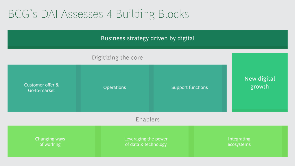
BCG Digital Acceleration Index
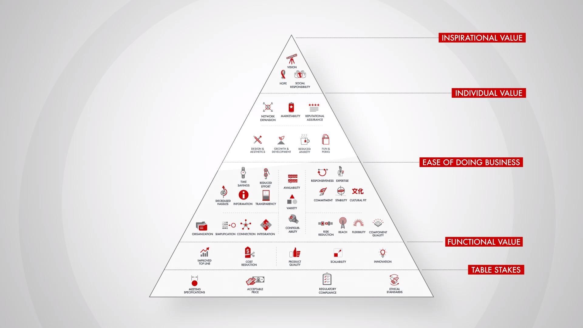
Bain’s Elements of Value Framework
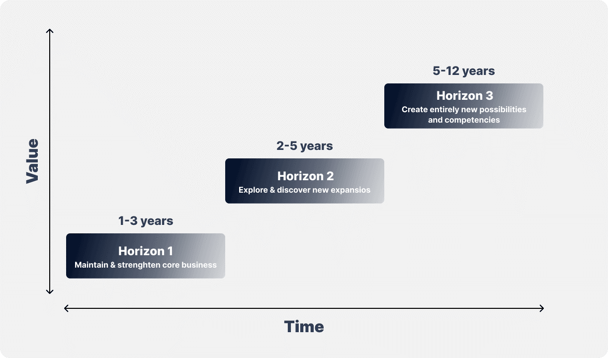
McKinsey Growth Pyramid
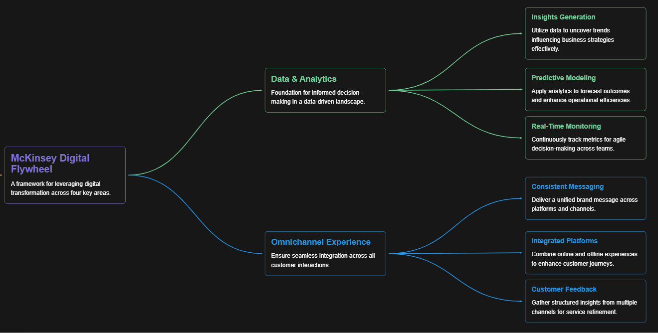
McKinsey Digital Flywheel

McKinsey 9-Box Talent Matrix

McKinsey 7S Framework

The Psychology of Persuasion in Marketing

The Influence of Colors on Branding and Marketing Psychology

What is Marketing?
Recent Blogs

Part 8: From Blocks to Brilliance – How Transformers Became Large Language Models (LLMs) of the series - From Sequences to Sentience: Building Blocks of the Transformer Revolution

Part 7: The Power of Now – Parallel Processing in Transformers of the series - From Sequences to Sentience: Building Blocks of the Transformer Revolution
Part 6: The Eyes of the Model – Self-Attention of the series - From Sequences to Sentience: Building Blocks of the Transformer Revolution

Part 5: The Generator – Transformer Decoders of the series - From Sequences to Sentience: Building Blocks of the Transformer Revolution

Part 4: The Comprehender – Transformer Encoders of the series - From Sequences to Sentience: Building Blocks of the Transformer Revolution of the series - From Sequences to Sentience: Building Blocks of the Transformer Revolution