Binomial Distribution
The binomial distribution is a widely used discrete probability distribution in statistics. Unlike the normal distribution, which is continuous, the binomial distribution models the likelihood of obtaining 'x' successes in 'n' trials, given that each trial has a fixed probability 'p' of success.
Key Concepts:
- A single experiment with only two possible outcomes (success/failure) is known as a Bernoulli trial.
- A sequence of independent Bernoulli trials forms a Bernoulli process.
- If an experiment consists of n independent trials where each trial results in a success (with probability p) or a failure (with probability q = 1 - p), the number of successes follows a binomial distribution.
- When n = 1, the binomial distribution simplifies to a Bernoulli distribution.
Binomial Distribution Formula
For a discrete random variable X, representing the number of successes in n independent trials, the probability mass function (PMF) is given by:

where:
- n = total number of trials
- k = number of successful outcomes
- p = probability of success in each trial
- (1 - p) = probability of failure
- (n! / (k!(n - k)!)) represents the binomial coefficient.
Binomial Distribution Mean and Variance
For a binomial distribution, the mean, variance and standard deviation for the given number of success are represented using the formulas
Mean, μ = np
Variance, σ2 = npq
Standard Deviation σ= √(npq)
Where p is the probability of success
q is the probability of failure, where q = 1-p
Binomial Distribution vs. Normal Distribution
The key distinction between the binomial distribution and the normal distribution is that the binomial distribution is discrete, while the normal distribution is continuous. The binomial distribution consists of a finite number of events, whereas the normal distribution represents an infinite number of possibilities. However, when the sample size of a binomial distribution is large, its probability curve closely resembles that of a normal distribution.
Characteristics of Binomial Distribution
The binomial distribution has the following key properties:
- It consists of two possible outcomes: success or failure, true or false, yes or no.
- The number of trials (n) is fixed, and each trial is independent.
- The probability of success (p) remains constant across all trials.
- Only the number of successes is counted in the given trials.
- The outcome of one trial does not influence the outcome of another.
Real-World Applications of Binomial Distribution
The binomial distribution is used in various scenarios where each trial results in one of two outcomes—success or failure—and all trials are independent. Below are some common applications:
Medical Research & Clinical Trials
- Use Case: Used in clinical trials to estimate the probability of success (e.g., patients recovering after treatment).
- Example: If 10 patients take a new drug and the probability of a successful treatment is 0.7, the binomial distribution helps estimate the likelihood of at least 7 recoveries.
- Impact: Helps medical researchers evaluate treatment effectiveness.
Quality Control in Manufacturing
- Use Case: Used to model the likelihood of defective products in production lines.
- Example: If a factory produces light bulbs with a 1% defect rate and inspects 100 bulbs, the binomial distribution helps estimate how many defective units are likely.
- Impact: Assists manufacturers in maintaining product quality and minimizing defects.
Marketing and A/B Testing
- Use Case: Used to analyze the effectiveness of marketing campaigns or website optimizations.
- Example: If a website has a conversion rate of 5%, the binomial distribution can estimate the likelihood of a certain number of conversions out of 200 visitors.
- Impact: Enables marketers to refine strategies based on data-driven insights.
Sports Analytics
- Use Case: Used to predict success rates in sports events, such as the number of goals scored or free throws made.
- Example: If a basketball player has a 75% free-throw success rate, the binomial distribution helps determine the probability of making 8 out of 10 shots.
- Impact: Helps coaches and analysts assess player performance and strategy.
Elections and Polling
- Use Case: Used to predict election outcomes based on voter support.
- Example: If a candidate has a 60% chance of winning each vote, the binomial distribution estimates the probability of getting a majority in a sample of 1,000 votes.
- Impact: Aids in forecasting election results and public opinion trends.
Genetics and Inheritance
- Use Case: Used to model the likelihood of inheriting a gene or genetic trait.
- Example: If a recessive gene has a 25% probability of being passed on, the binomial distribution estimates how many out of 10 offspring will inherit it.
- Impact: Assists geneticists in predicting hereditary traits and probabilities.
Importance of Binomial Distribution
The binomial distribution is fundamental in probability and statistics for several reasons:
Binary Event Modeling
- Relevance: Ideal for scenarios involving two possible outcomes (success/failure), such as product quality checks, election forecasting, and customer behavior analysis.
- Example: Used to determine the probability of getting a certain number of heads in a series of coin flips.
Foundation for Statistical Tests
- Relevance: Serves as the basis for binomial hypothesis testing, which is used to analyze sample proportions.
- Example: In quality control, hypothesis testing helps determine whether the proportion of defective products exceeds acceptable limits.
Bernoulli Trials & Independence
- Relevance: Built upon independent Bernoulli trials, making it a fundamental concept in probability theory.
- Example: Used to model independent outcomes, such as answering multiple-choice questions correctly or rolling dice.
Cumulative Probability Calculation
- Relevance: Allows calculation of probabilities for cumulative successes, such as "What is the probability of at least 5 successes?"
- Example: In business, estimating the probability of reaching a minimum number of sales helps in setting targets.
Connection to the Normal Distribution
- Relevance: When the number of trials (n) is large, the binomial distribution approximates a normal distribution (per the Central Limit Theorem).
- Example: In a large dataset (e.g., 1,000 coin flips), the binomial distribution's probability curve closely resembles that of a normal distribution, simplifying analysis.
Practical Applications Across Industries
- Relevance: Widely used in diverse fields such as finance, medicine, engineering, and marketing, making it a key statistical tool.
- Example: Helps businesses predict consumer behavior, assists in reliability testing, and improves quality assurance processes.
Implementation of Binomial Distribution:
import numpy as np
import matplotlib.pyplot as plt
from scipy.stats import binom

# Parameters for the binomial distribution
n_trials = 10     # Number of trials (e.g., flipping a coin 10 times)
p_success = 0.5   # Probability of success in each trial (e.g., probability of heads in a coin flip)

# Generating a binomial random variable
x = np.arange(0, n_trials + 1)  # Possible outcomes (0 to n_trials successes)
pmf = binom.pmf(x, n_trials, p_success)  # Probability mass function (PMF)

# Plotting the Binomial Distribution (PMF)
plt.figure(figsize=(8, 6))
plt.bar(x, pmf, color='blue', alpha=0.7)
plt.title(f'Binomial Distribution: n={n_trials}, p={p_success}')
plt.xlabel('Number of Successes')
plt.ylabel('Probability')
plt.show()

# Sample 1000 outcomes from the binomial distribution
n_samples = 1000
samples = binom.rvs(n_trials, p_success, size=n_samples)

# Plotting the histogram of the sampled data
plt.figure(figsize=(8, 6))
plt.hist(samples, bins=np.arange(-0.5, n_trials + 1.5, 1), density=True, color='green', alpha=0.7, rwidth=0.8)
plt.title(f'Sampled Binomial Distribution: n={n_trials}, p={p_success}')
plt.xlabel('Number of Successes')
plt.ylabel('Relative Frequency')
plt.show()

# Mean and variance of the binomial distribution
mean, var = binom.stats(n_trials, p_success)

print(f"Mean of binomial distribution: {mean:.2f}")
print(f"Variance of binomial distribution: {var:.2f}")

# Probability of getting exactly 5 successes
prob_5_successes = binom.pmf(5, n_trials, p_success)
print(f"Probability of exactly 5 successes: {prob_5_successes:.4f}")

# Cumulative probability of getting 6 or fewer successes
cum_prob_6_or_fewer = binom.cdf(6, n_trials, p_success)
print(f"Cumulative probability of 6 or fewer successes: {cum_prob_6_or_fewer:.4f}")
Mean of binomial distribution: 5.00
Variance of binomial distribution: 2.50
Probability of exactly 5 successes: 0.2461
Cumulative probability of 6 or fewer successes: 0.8281


Conclusion:
The binomial distribution is a key concept in probability and statistics, serving as a foundation for analyzing binary outcomes and facilitating statistical inference across various fields. Its significance stems from its straightforward nature, strong alignment with real-world scenarios, and its role in shaping the understanding of more advanced distributions like the normal distribution. From healthcare and manufacturing to marketing and sports analytics, the binomial distribution is an essential tool for making informed decisions in uncertain conditions.
Featured Blogs
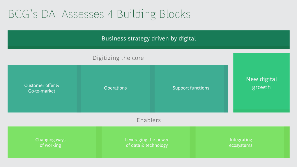
BCG Digital Acceleration Index

Bain’s Elements of Value Framework
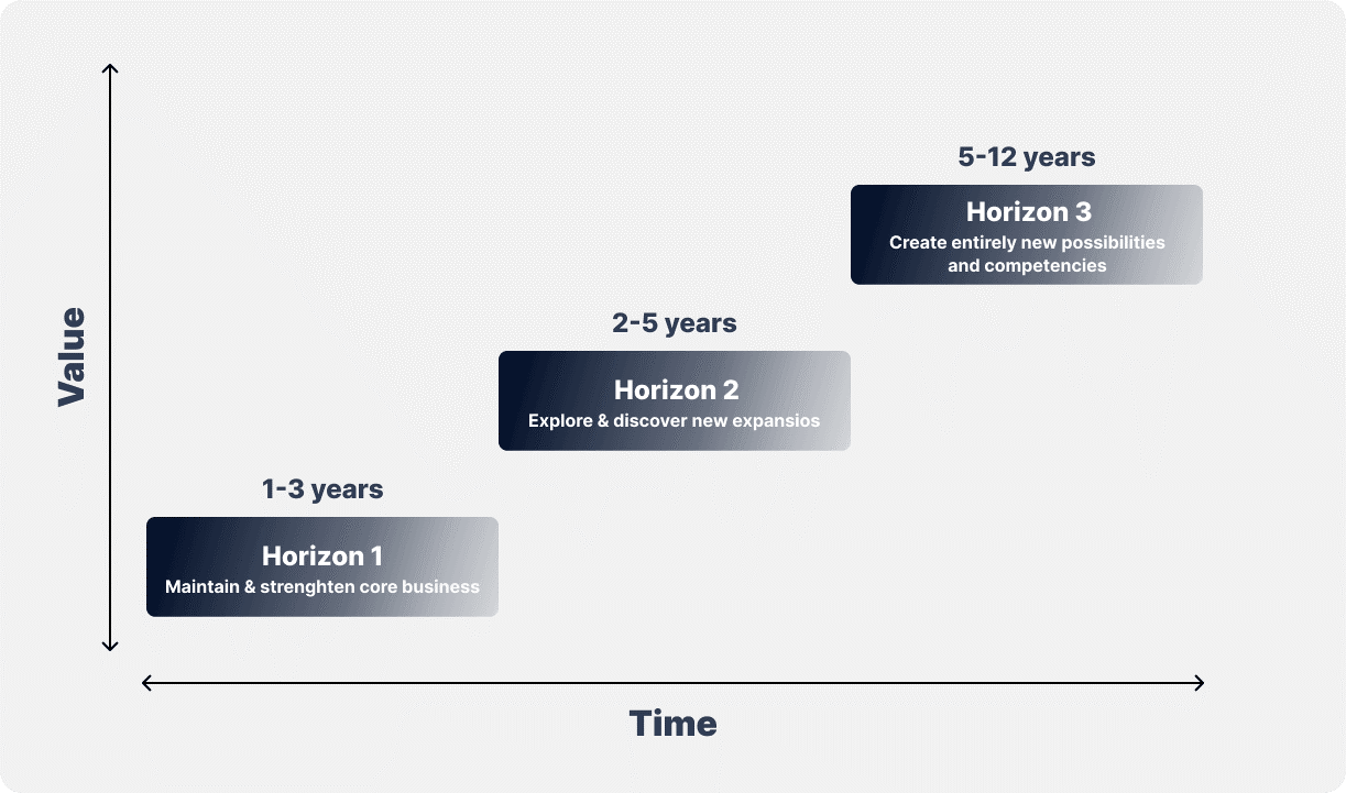
McKinsey Growth Pyramid
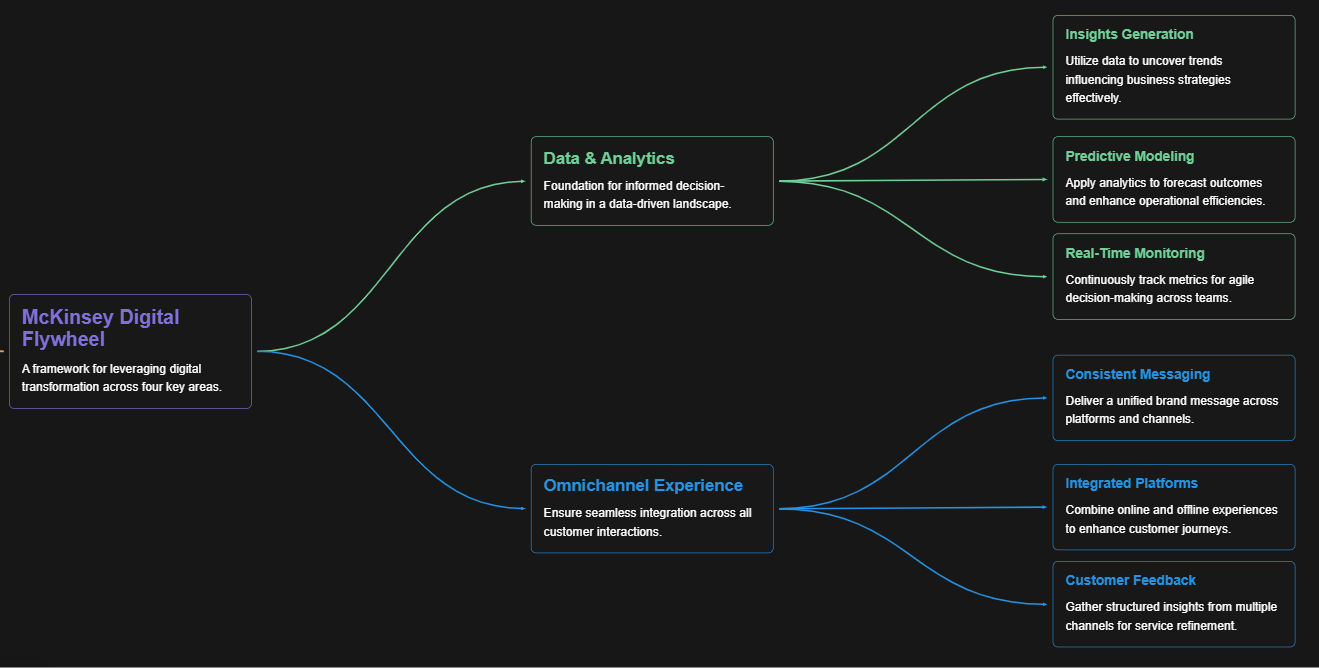
McKinsey Digital Flywheel

McKinsey 9-Box Talent Matrix

McKinsey 7S Framework

The Psychology of Persuasion in Marketing

The Influence of Colors on Branding and Marketing Psychology

What is Marketing?
Recent Blogs

Part 8: From Blocks to Brilliance – How Transformers Became Large Language Models (LLMs) of the series - From Sequences to Sentience: Building Blocks of the Transformer Revolution

Part 7: The Power of Now – Parallel Processing in Transformers of the series - From Sequences to Sentience: Building Blocks of the Transformer Revolution
Part 6: The Eyes of the Model – Self-Attention of the series - From Sequences to Sentience: Building Blocks of the Transformer Revolution

Part 5: The Generator – Transformer Decoders of the series - From Sequences to Sentience: Building Blocks of the Transformer Revolution

Part 4: The Comprehender – Transformer Encoders of the series - From Sequences to Sentience: Building Blocks of the Transformer Revolution of the series - From Sequences to Sentience: Building Blocks of the Transformer Revolution