Beta Distribution
The Beta Distribution is a family of continuous probability distributions that exist within the range [0,1][0,1][0,1]. It is primarily used for modeling probabilities and proportions, making it an essential tool in fields such as business analytics, Bayesian statistics, and quality control. Due to its flexibility, the Beta distribution is widely applied in scenarios where likelihood estimation is crucial.
Table of Contents:
- Definition
- Probability Density Function (PDF)
- Formula
- Graph and Shapes of Beta Distribution
- Cumulative Distribution Function (CDF)
- Key Properties
- Mean and Variance
- Relationship with Other Distributions
- Applications and Significance
- Python Implementation
- Conclusion
1. Understanding the Beta Distribution
The Beta Distribution is a continuous probability distribution defined by two positive shape parameters:
- α\alphaα (alpha): Often interpreted as the "success" parameter.
- β\betaβ (beta): Often considered the "failure" parameter.
These parameters influence the overall shape of the distribution, making it highly adaptable. Depending on the values of α\alphaα and β\betaβ, the distribution can exhibit a variety of forms, from uniform to highly skewed. The Beta distribution is particularly useful for modeling probabilities or proportions in uncertain environments.
2. Probability Density Function (PDF)
The probability density function of a Beta-distributed variable XXX, parameterized by α\alphaα and β\betaβ, is defined as:
![]()
Beta Function:
Graph and Shape of the Beta Distribution
The shape of the Beta distribution varies significantly depending on the values of the parameters 𝛼 and 𝛽:
- Symmetric Form: When 𝛼 and 𝛽 are equal (𝛼 = 𝛽), the distribution remains symmetric. Specifically, if 𝛼 = 𝛽 = 1, it simplifies to a uniform distribution over the interval [0,1].
- Right-Skewed: If 𝛼 is smaller than 𝛽 (𝛼 < 𝛽), the probability mass is concentrated towards 0, making the distribution skewed to the right.
- Left-Skewed: When 𝛼 is greater than 𝛽 (𝛼 > 𝛽), the distribution leans towards 1, resulting in a left-skewed shape.
- Highly Peaked: If both 𝛼 and 𝛽 have large values, the distribution is sharply concentrated around its mean, forming a distinct peak.
Cumulative Distribution Function (CDF)
The cumulative distribution function (CDF) of the Beta distribution is expressed using the incomplete Beta function. Since its computation is complex, it is typically evaluated using specialized software or reference tables.
The CDF for a Beta-distributed random variable XXX with parameters α\alphaα and β\betaβ is given by:

Properties of the Beta Distribution
The Beta distribution possesses several notable characteristics:
- Bounded Range: The distribution is always constrained within the interval [0,1].
- Versatility: By adjusting the shape parameters α (alpha) and β (beta), the Beta distribution can adopt various forms, making it highly adaptable.
- Symmetry: When α = β, the distribution is symmetric around 0.5.
- Additive Property: If multiple independent Beta-distributed variables share the same β parameter but have different α parameters, their sum also follows a Beta distribution.
Mean and Variance
For a Beta distribution with parameters α and β, the mean and variance are given by:
Mean:
![]()
Variance:

Impact of Mean and Variance
The formulas for mean and variance illustrate how the relative values of α (alpha) and β (beta) influence the central tendency and dispersion of the distribution.
Connections with Other Distributions
The Beta distribution has significant relationships with other probability distributions:
- Uniform Distribution: When α = β = 1, the Beta distribution simplifies to a uniform distribution over the interval [0,1].
- Bernoulli and Binomial Distributions: In Bayesian statistics, the Beta distribution serves as the conjugate prior for Bernoulli and binomial distributions, making it useful for probabilistic inference.
- Dirichlet Distribution: The Beta distribution is a specific case of the Dirichlet distribution, which generalizes it for multiple categorical outcomes.
Applications of the Beta Distribution
The Beta distribution is particularly useful for modeling variables restricted between 0 and 1, making it widely applicable in various fields:
1. Bayesian Inference
- Prior and Posterior Distributions: In Bayesian analysis, the Beta distribution represents prior beliefs about probabilities, which are updated with new data to form posterior distributions.
- A/B Testing: It plays a crucial role in estimating conversion rates, success probabilities, and response rates, enabling data-driven decision-making.
2. Probability and Proportion Modeling
- Estimating Success Rates: The Beta distribution is used in fields like quality control and product testing to model the probability of binary outcomes (e.g., defect rates in manufacturing).
- Machine Learning Applications: It is applied in probabilistic models to estimate classification probabilities or feature distributions.
3. Marketing and Consumer Behavior Analysis
- Customer Engagement Metrics: The Beta distribution helps model customer response rates, conversion probabilities, and engagement levels.
- Campaign Performance Estimation: Marketers use it to track the effectiveness of advertising efforts by quantifying success and failure rates.
4. Reliability Engineering and Failure Analysis
- Component Reliability Assessment: Engineers use the Beta distribution to estimate the likelihood of success or failure, particularly when data is scarce.
- Predicting Failure Rates: By adjusting parameters based on prior knowledge, it helps in assessing product longevity and reliability.
5. Educational Testing and Psychometrics
- Score Probabilities in Testing: The Beta distribution is applied in psychometric models to estimate student performance probabilities.
- Adaptive Testing: It helps define score distributions in computer-based adaptive assessments.
Importance of the Beta Distribution
The Beta distribution is valuable due to its ability to effectively model probabilities and proportions within a bounded range [0,1]. Key advantages include:
- Suitability for Bounded Data: Unlike many other distributions, it naturally models data constrained between 0 and 1, making it ideal for proportions and probabilities.
- Significance in Bayesian Analysis: As a conjugate prior for binomial distributions, it plays a vital role in Bayesian updating, allowing data-driven adjustments to probability estimates.
- Adaptability for Real-World Applications: Its shape parameters enable precise modeling of probabilities in diverse fields such as marketing, finance, and quality assurance.
By adjusting α and β, the Beta distribution can model a broad range of probability distributions, from uniform to highly skewed, making it an essential tool in statistical modeling and decision-making.
Python Implementation
import numpy as np
import scipy.stats as stats
import matplotlib.pyplot as plt

# Setting up for better visualization
plt.style.use('seaborn-darkgrid')
The Beta distribution has two main parameters:
Alpha (α): Often referred to as the "shape" parameter; it controls the shape of the distribution.
Beta (β): Another "shape" parameter that also influences the distribution.
# Define range for x-axis (the Beta distribution is defined over [0, 1])
x = np.linspace(0, 1, 500)

# Beta distribution with various alpha and beta parameters
alpha_values = [0.5, 2, 5]  # Different alpha parameters
beta_values = [0.5, 2, 5]   # Different beta parameters

# Plotting the Beta PDF with varying alpha parameters
fig, ax = plt.subplots(figsize=(10, 6))
for alpha in alpha_values:
    y = stats.beta.pdf(x, a=alpha, b=2)  # Fixing beta to 2
    ax.plot(x, y, label=f'alpha={alpha}, beta=2')

ax.set_title('Beta PDF with Varying Alpha Parameter')
ax.set_xlabel('x')
ax.set_ylabel('Probability Density')
ax.legend()
plt.show()

The plot above demonstrates how varying alpha affects the shape of the distribution, with smaller values creating a U-shape and higher values concentrating density near the right edge of the interval.
Exploring the Effect of the Beta Parameter
Now let’s examine how changing the beta parameter affects the distribution while keeping alpha constant.
# Plotting the Beta PDF with varying beta parameters
fig, ax = plt.subplots(figsize=(10, 6))
for beta in beta_values:
    y = stats.beta.pdf(x, a=2, b=beta)  # Fixing alpha to 2
    ax.plot(x, y, label=f'alpha=2, beta={beta}')

ax.set_title('Beta PDF with Varying Beta Parameter')
ax.set_xlabel('x')
ax.set_ylabel('Probability Density')
ax.legend()
plt.show()

In this plot, you can see that varying beta shapes the distribution differently, with lower values concentrating density near the left and higher values pulling density towards the right edge of the interval.
Beta Cumulative Distribution Function (CDF)
The CDF shows the cumulative probability up to a specific value. Here, we plot the CDF for different values of alpha and beta.
# Plotting Beta CDF with varying alpha parameters
fig, ax = plt.subplots(figsize=(10, 6))
for alpha in alpha_values:
    y = stats.beta.cdf(x, a=alpha, b=2)  # Fixing beta to 2
    ax.plot(x, y, label=f'alpha={alpha}, beta=2')

ax.set_title('Beta CDF with Varying Alpha Parameter')
ax.set_xlabel('x')
ax.set_ylabel('Cumulative Probability')
ax.legend()
plt.show()

The CDF plot helps illustrate the rate at which the cumulative probability approaches 1 for various alpha values.
Mean and Variance of the Beta Distribution
# Displaying mean and variance for different alpha and beta values
print("Beta Distribution Mean and Variance")
for alpha in alpha_values:
    for beta in beta_values:
        mean = alpha / (alpha + beta)
        variance = (alpha * beta) / ((alpha + beta)**2 * (alpha + beta + 1))
        print(f"Alpha={alpha}, Beta={beta} -> Mean={mean:.2f}, Variance={variance:.2f}")
These calculations give us insights into the central tendency and spread of the distribution based on different parameter combinations.
Real-World Application Example: Modeling Probability of Success
Let’s use the Beta distribution to model a scenario where we observe the proportion of successful outcomes in a binomial experiment (e.g., customer purchase rate). We can plot both the PDF and CDF to understand the distribution of probabilities.
alpha = 5  # Shape parameter representing "successes"
beta = 3   # Shape parameter representing "failures"

# Probability Density Function
fig, ax = plt.subplots(1, 2, figsize=(14, 6))

# PDF
y_pdf = stats.beta.pdf(x, a=alpha, b=beta)
ax[0].plot(x, y_pdf, color='b')
ax[0].set_title('Beta PDF for Modeling Success Probability')
ax[0].set_xlabel('Probability of Success')
ax[0].set_ylabel('Probability Density')

# CDF
y_cdf = stats.beta.cdf(x, a=alpha, b=beta)
ax[1].plot(x, y_cdf, color='g')
ax[1].set_title('Beta CDF for Modeling Success Probability')
ax[1].set_xlabel('Probability of Success')
ax[1].set_ylabel('Cumulative Probability')

plt.show()

The PDF shows the likelihood of different probabilities for success, while the CDF provides the cumulative probability, useful for estimating the probability of success up to a certain threshold.
Sampling from a Beta Distribution
Now, let’s generate random samples from the Beta distribution and visualize the histogram to see how it aligns with the theoretical PDF.
# Generating samples and plotting histogram with PDF overlay
samples = np.random.beta(alpha, beta, size=1000)

fig, ax = plt.subplots(figsize=(10, 6))
# Histogram of samples
ax.hist(samples, bins=30, density=True, alpha=0.6, color='skyblue', label='Sampled Data')
# Overlaying PDF
ax.plot(x, stats.beta.pdf(x, a=alpha, b=beta), color='red', lw=2, label='Theoretical PDF')
ax.set_title(f'Beta Distribution Samples and PDF Overlay\n(alpha={alpha}, beta={beta})')
ax.set_xlabel('Value')
ax.set_ylabel('Density')
ax.legend()
plt.show()

Conclusion
The Beta distribution is a crucial tool for modeling data restricted to the 0 to 1 range, including probabilities, proportions, and rates. It is particularly valuable in fields where probability estimates must be continuously updated. Serving as a conjugate prior in Bayesian analysis, it facilitates belief updates as new data becomes available, making it widely used in A/B testing, marketing analytics, and quality control. Its adaptability allows for precise representation of real-world probabilities, such as customer engagement rates and defect proportions. The Beta distribution's strength lies in its ability to effectively model bounded probabilistic data, making it indispensable for applications that require accurate probability estimation and data-driven decision-making.
Featured Blogs

BCG Digital Acceleration Index

Bain’s Elements of Value Framework
McKinsey Growth Pyramid
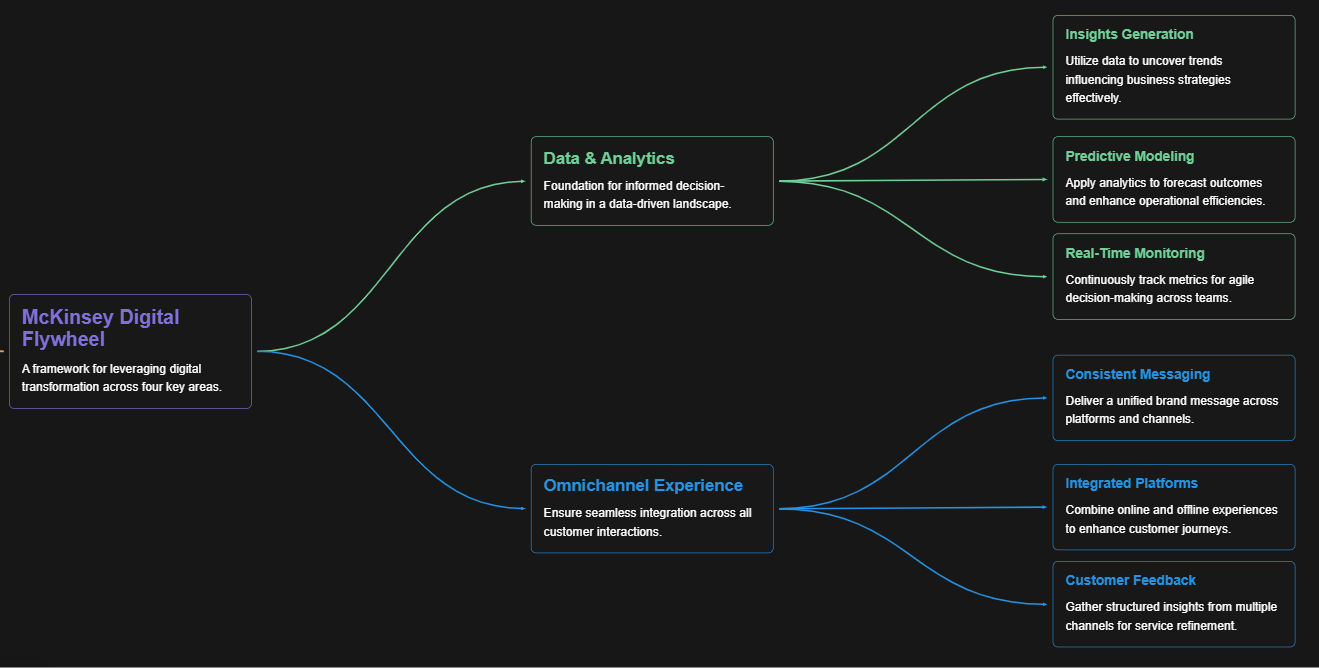
McKinsey Digital Flywheel

McKinsey 9-Box Talent Matrix

McKinsey 7S Framework

The Psychology of Persuasion in Marketing

The Influence of Colors on Branding and Marketing Psychology

What is Marketing?
Recent Blogs

Part 8: From Blocks to Brilliance – How Transformers Became Large Language Models (LLMs) of the series - From Sequences to Sentience: Building Blocks of the Transformer Revolution

Part 7: The Power of Now – Parallel Processing in Transformers of the series - From Sequences to Sentience: Building Blocks of the Transformer Revolution

Part 6: The Eyes of the Model – Self-Attention of the series - From Sequences to Sentience: Building Blocks of the Transformer Revolution

Part 5: The Generator – Transformer Decoders of the series - From Sequences to Sentience: Building Blocks of the Transformer Revolution

Part 4: The Comprehender – Transformer Encoders of the series - From Sequences to Sentience: Building Blocks of the Transformer Revolution of the series - From Sequences to Sentience: Building Blocks of the Transformer Revolution