
Bayesian Statistics
Bayesian statistics is a statistical approach based on Bayes' Theorem, which provides a mathematical framework for updating probabilities as new data emerges. Unlike traditional frequentist methods, Bayesian statistics incorporates prior knowledge (prior probability) and refines it with observed data (likelihood) to derive a posterior probability. This iterative process makes Bayesian methods particularly useful in situations involving uncertainty and evolving information.
Table of Contents
- Introduction to Bayesian Statistics
- Bayes’ Theorem
- Formula and Explanation
- Example
- Key Concepts in Bayesian Statistics
- Credible Intervals
- Conjugate Priors
- Bayesian Networks
- Importance of Bayesian Statistics
- Applications of Bayesian Statistics
- Implementation in Python
- Conclusion
Introduction to Bayesian Statistics
Bayesian statistics is an approach to probability that defines probability as a measure of belief in an event, rather than just a frequency of occurrence. This perspective contrasts with the frequentist approach, which interprets probability as the long-run frequency of an event occurring in repeated trials. In Bayesian analysis, prior knowledge is represented as a probability distribution (prior distribution), which is then updated using Bayes' Theorem as new data becomes available.
Bayesian methods apply this theorem to update beliefs and estimate parameters in statistical models. Since Bayesian probability is interpreted as a degree of belief, it allows for direct probability assignments to parameters, providing a flexible framework for inference and decision-making.
Bayes’ Theorem Formula
Bayes’ Theorem offers a structured approach to revising probabilities in light of new evidence. The formula is:
![]()
Where,
P(A|B): Posterior probability - The probability of event A occurring given that B is true.
P(B∣A): Likelihood - The probability of event B occurring given that A is true.
P(A): Prior probability - The initial probability of event A before observing event B.
P(B) Marginal probability - The total probability of event B occurring.
Explanation
Bayes' Theorem helps update the probability of an event (A) based on new evidence (B).
- Prior Probability (P(A)):
This is the initial probability of an event occurring before any additional data is considered. - Likelihood (P(B | A)):
This represents the probability of observing evidence B, assuming event A is true. - Marginal Probability (P(B)):
This is the total probability of observing evidence B, considering all possible causes. - Posterior Probability (P(A | B)):
This is the revised probability of event A occurring after incorporating the new evidence B.
Example
A clinic conducts a test for a disease that affects 1% of the population (P(Disease) = 0.01). The test correctly detects the disease 95% of the time (P(Test | Disease) = 0.95) but has a false positive rate of 5% (P(Test | No Disease) = 0.05).
What is the probability that a person actually has the disease given that they tested positive?
Using Bayes' Theorem:
Formula in Unicode:

Where:
𝑃(𝐷𝑖𝑠𝑒𝑎𝑠𝑒) = 0.01 (prior probability)
𝑃(𝑇𝑒𝑠𝑡 ∣ 𝐷𝑖𝑠𝑒𝑎𝑠𝑒) = 0.95 (likelihood)
𝑃(𝑇𝑒𝑠𝑡) can be computed as:
𝑃(𝑇𝑒𝑠𝑡) = 𝑃(𝑇𝑒𝑠𝑡 ∣ 𝐷𝑖𝑠𝑒𝑎𝑠𝑒) ⋅ 𝑃(𝐷𝑖𝑠𝑒𝑎𝑠𝑒) + 𝑃(𝑇𝑒𝑠𝑡 ∣ 𝑁𝑜𝐷𝑖𝑠𝑒𝑎𝑠𝑒) ⋅ 𝑃(𝑁𝑜𝐷𝑖𝑠𝑒𝑎𝑠𝑒)
𝑃(𝑇𝑒𝑠𝑡) = (0.95 × 0.01) + (0.05 × 0.99)
P ( Test) ≈ 0.059
Interpretation:
If an individual receives a positive test result, there is approximately a 16.1% probability that they actually have the disease, considering the test's accuracy and the disease's prevalence in the population.
Key Concepts in Bayesian Statistics
1. Credible Intervals
- A Bayesian interval estimate that provides a range within which a parameter is likely to fall with a specified probability (e.g., 95%).
- Based on the posterior distribution, offering a direct measure of uncertainty regarding the parameter.
- Example: "There is a 95% probability that the parameter lies within the interval [a,b][a, b][a,b]."
2. Conjugate Priors
- A prior distribution is considered conjugate if the resulting posterior distribution belongs to the same family as the prior distribution, making computations more straightforward.
- Example: When a Beta distribution is used as a prior for a Binomial likelihood, the resulting posterior distribution is also Beta.
- Conjugate priors are beneficial for deriving analytical solutions in Bayesian inference.
3. Bayesian Networks
- A probabilistic graphical model that represents variables as nodes and their dependencies as directed edges.
- It describes conditional dependencies between variables using joint probability distributions.
- Applications: Medical diagnosis, anomaly detection, and decision-making.
- Example: Smoking → Lung Cancer → Coughing.
Importance of Bayesian Statistics
- Utilization of Prior Information: Allows the integration of expert insights or historical data into statistical analysis.
- Continuous Updating: Adjusts probability estimates dynamically as new data becomes available, making it essential for real-time decision-making.
- Intuitive Probability Interpretation: Represents outcomes as probabilities, making decision-making under uncertainty more straightforward.
- Versatile Modeling Approach: Effectively manages complex scenarios, including missing data, hierarchical structures, and non-traditional distributions.
- Broad Range of Applications: Extensively used across various fields, including healthcare, finance, artificial intelligence, and more.
Real-World Applications of Bayesian Statistics
- Machine Learning: Forms the foundation of techniques such as Naïve Bayes classifiers, Bayesian networks, and Bayesian optimization.
- Healthcare: Applied in disease diagnosis, clinical trials, and personalized treatment strategies.
- Finance: Used for portfolio management, fraud detection, and predictive analytics.
- Marketing and A/B Testing: Enhances campaign performance by dynamically updating success probabilities.
- Environmental Science: Helps in forecasting weather patterns and assessing climate change impacts.
- Supply Chain & Logistics: Aids in demand forecasting and inventory optimization.
Implementation in Python
Simple Bayesian Interface

Bayesian Linear Regression with PyMC3

Conclusion
Bayesian statistics provides a robust approach to probabilistic reasoning, allowing beliefs to be updated dynamically as new evidence emerges. Its ability to incorporate prior knowledge and adapt to changing data makes it a valuable tool across various domains, including machine learning and healthcare. By utilizing specialized tools such as Python libraries (e.g., PyMC3), professionals can effectively apply Bayesian methods to extract meaningful insights and enhance decision-making in uncertain environments.
Featured Blogs

BCG Digital Acceleration Index

Bain’s Elements of Value Framework
McKinsey Growth Pyramid
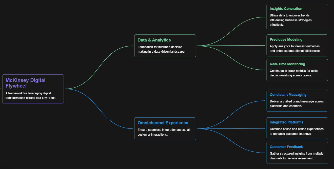
McKinsey Digital Flywheel

McKinsey 9-Box Talent Matrix

McKinsey 7S Framework

The Psychology of Persuasion in Marketing

The Influence of Colors on Branding and Marketing Psychology

What is Marketing?
Recent Blogs

Part 8: From Blocks to Brilliance – How Transformers Became Large Language Models (LLMs) of the series - From Sequences to Sentience: Building Blocks of the Transformer Revolution

Part 7: The Power of Now – Parallel Processing in Transformers of the series - From Sequences to Sentience: Building Blocks of the Transformer Revolution

Part 6: The Eyes of the Model – Self-Attention of the series - From Sequences to Sentience: Building Blocks of the Transformer Revolution

Part 5: The Generator – Transformer Decoders of the series - From Sequences to Sentience: Building Blocks of the Transformer Revolution

Part 4: The Comprehender – Transformer Encoders of the series - From Sequences to Sentience: Building Blocks of the Transformer Revolution of the series - From Sequences to Sentience: Building Blocks of the Transformer Revolution